
Heuristic Techniques in Biological Sequence Alignment: Banded DP and FASTA
E N D
Presentation Transcript
Sequence Alignment IILecture #3 Background Readings: Chapters 2.5, 2.7 in the text book, Biological Sequence Analysis, Durbin et al., 2001. Chapters 3.5.1- 3.5.3, 3.6.2 in Introduction to Computational Molecular Biology, Setubal and Meidanis, 1997. This class has been edited from Nir Friedman’s lecture which is available at www.cs.huji.ac.il/~nir. Changes made by Dan Geiger, then by Shlomo Moran. .
Reminder • Last class we discussed dynamic programming algorithms for • global alignment • local alignment • All of these assumed a scoring rule:that determines the quality of perfect matches, substitutions, insertions, and deletions.
Alignment in Real Life • One of the major uses of alignments is to find sequences in a “database.” • The current protein database contains about 100 millions (i.e.,108) residues ! So searching a 1000 long target sequence requires to evaluate about 1011 matrix cells which will take about three hours in the rate of 10 millions evaluations per second. • Quite annoying when, say, one thousand target sequences need to be searched because it will take about four months to run.
Heuristic Fast Search • Instead, most searches rely on heuristic procedures • These are not guaranteed to find the best match • Sometimes, they will completely miss a high-scoring match We now describe the main ideas used by the best known of these heuristic procedures.
Basic Intuition • Almost all heuristic search procedures are based on the observation that real-life matches often contain long strings with gap-less matches. • These heuristic try to find significant gap-less matches and then extend them.
Banded DP • Suppose that we have two strings s[1..n] and t[1..m] such that nm • If the optimal alignment of s and t has few gaps, then path of the alignment will be close to diagonal s t
s k t V[i,i+k/2] V[i, i+k/2+1] Out of range V[i+1, i+k/2 +1] Note that for diagonals i-j = constant. Banded DP • To find such a path, it suffices to search in a diagonal region of the matrix. • If the diagonal band has width k, then the dynamic programming step takes O(kn). • Much faster than O(n2) of standard DP.
s k t Banded DP for local alignment Problem: Where is the banded diagonal ? It need not be the main diagonal when looking for a good local alignment. How do we select which subsequences to align using banded DP? We heuristically find potential diagonals and evaluate them using Banded DP. This is the main idea of FASTA.
Finding Potential Diagonals Suppose that we have a relatively long gap-less match AGCGCCATGGATTGAGCGA TGCGACATTGATCGACCTA • Can we find “clues” that will let us find it quickly? • Each such sequence defines a potential diagonal (which is then evaluated using Banded DP.
s t Signature of a Match Assumption: good matches contain several “patches” of perfect matches AGCGCCATGGATTGAGCTA TGCGACATTGATCGACCTA Since this is a gap-less alignment, all perfect match regionsshould be on one diagonal
s t FASTA-finding ungapped matches Input: strings s and t, and a parameter ktup • Find all pairs (i,j) such that s[i..i+ktup]=t[j..j+ktup] • Locate sets of pairs that are on the same diagonal • By sorting according to the difference i-j • Compute the score for the diagonal that contains all these pairs
s t FASTA-finding ungapped matches Input: strings s and t, and a parameter ktup • Find all pairs (i,j) such that s[i..i+ktup]=t[j..j+ktup] • Step one: prepare an index of the database such that given a sequence of length ktup, one gets the list of positions. (Linear time). • Step two: run on all sequences of size ktup on the query sequence. ( time depends on # of positions).
s 2 t 3 1 FASTA- using banded DP Final steps: • List the highest scoring diagonal matches • Run banded DP on the region containing any high scoring diagonal (say with width 12). Hence, the algorithm may combine some diagonals into gapped matches (in the example below combine diagonals 2 and 3).
s t FASTA- practical choices Most applications of FASTA use very small ktup (1-2 for proteins, and 4-6 for DNA). Higher values are faster, yielding less diagonal to search around, but increase the chance to miss the optimal local alignment. Some implementation choices /tricks have not been explicated herein.
FASTA-summary Input: strings s and t, and a parameter ktup =1,2,4,5, or 6 depending on the application. Output: A highly scored local alignment • Find pairs of matching substrings s[i..i+ktup]=t[j..j+ktup] • Extend to ungapped diagonals • Extend to gapped matches using banded DP
BLAST Overview(Basic Local Alignment Search Tool) Input: strings s and t, and a parameter T = threshold value Output: A highly scored local alignment Definition: Two strings s and t of length k are a high scoring pair (HSP) if d(s,t) > T (usually consider un-gapped alignments only). • Find high scoring pairs of substrings such that d(s,t) > T • These words serve as seeds for finding longer matches • Extend to ungapped diagonals (as in FASTA) • Extend to gapped matches
BLAST Overview (cont.) Step 1: Find high scoring pairs of substrings such that d(s,t) > T (The seeds): • Find all strings of length k which score at least T with substrings of s in a gapless alignment (k = 4 for proteins, 11 for DNA) (note: possibly, not all k-words must be tested, e.g. when such a word scores less than T with itself). • Find in t all exact matches with each of the above strings.
s t Extending Potential Matches Once a seed is found, BLAST attempts to find a local alignment that extends the seed. Seeds on the same diagonal are combined (as in FASTA), then extended as far as possible in a greedy manner. During the extension phase, the search stops when the score passes below some lower bound computed by BLAST (to save time).
Where do scoring rules come from ? We have defined an additive scoring function by specifying a function ( , ) such that • (x,y) is the score of replacing x by y • (x,-) is the score of deleting x • (-,x) is the score of inserting x But how do we come up with the “correct” score ? Answer: By encoding experience of what are similar sequences for the task at hand. Similarity depends on time, evolution trends, and sequence types.
Why use probability to define and/or interpret a scoring function ? • Similarity is probabilistic in nature because biological changes like mutation, recombination, and selection, are not deterministic. • We could answer questions such as: • How probable two sequences are similar? • Is the similarity found significant or random? • How to change a similarity score when, say, mutation rate of a specific area on the chromosome becomes known ?
A Probabilistic Model • For now, we will focus on alignment without indels. • For now, we assume each position (nucleotide /amino-acid) is independent of other positions. • We consider two options: M: the sequences are Matched(related) R: the sequences are Random (unrelated)
Unrelated Sequences • Our random model of unrelated sequences is simple • Each position is sampled independently from a distribution over the alphabet • We assume there is a distribution q() that describes the probability of letters in such positions. • Then:
Related Sequences • We assume that each pair of aligned positions (s[i],t[i]) evolved from a common ancestor • Let p(a,b) be a distribution over pairs of letters. • p(a,b) is the probability that some ancestral letter evolved into this particular pair of letters.
Odd-Ratio Test for Alignment If Q > 1, then the two strings s and t are more likely to be related (M) than unrelated (R). If Q < 1, then the two strings s and t are more likely to be unrelated (R) than related (M).
Log Odd-Ratio Test for Alignment Score(s[i],t[i]) Taking logarithm of Q yields If log Q > 0, then s and t are more likely to be related. If log Q < 0, then they are more likely to be unrelated. How can we relate this quantity to a score function ?
Probabilistic Interpretation of Scores • We define the scoring function via • Then, the score of an alignment is the log-ratio between the two models: • Score > 0 Model is more likely • Score < 0 Random is more likely
Modeling Assumptions • It is important to note that this interpretation depends on our modeling assumption!! • For example, if we assume that the letter in each position depends on the letter in the preceding position, then the likelihood ratio will have a different form.
Estimating Probabilities • Suppose we are given a long string s[1..n] of letters from • We want to estimate the distribution q(·) that generated the sequence • How should we go about this? We build on the theory of parameter estimation in statistics using either maximum likelihood estimation or the Bayesian approach .
Estimating q() • Suppose we are given a long string s[1..n] of letters from • s can be the concatenation of all sequences in our database • We want to estimate the distribution q() • That is, q is defined per letter Likelihood function:
Estimating q()(cont.) How do we define q? Likelihood function: ML parameters (Maximum Likelihood) MAP parameters (Maximum A posteriori Probability)
Estimating p(·,·) Intuition: • Find pair of aligned sequences s[1..n], t[1..n], • Estimate probability of pairs: • Again, s and t can be the concatenation of many aligned pairs from the database Number of times a is aligned with b in (s,t)
Problems in Estimating p(·,·) • How do we find pairs of aligned sequences? • How far is the ancestor ? • earlier divergence low sequence similarity • later divergence high sequence similarity • Does one letter mutate to the other or are they both mutations of a common ancestor having yet another residue/nucleotide acid ?