ChIP-seq
Institute for Computational Biomedicine. ChIP-seq. Olivier Elemento, PhD TA: Jenny Giannopoulou, PhD. CSHL High Throughput Data Analysis Workshop, June 2012. Plan. ChIP-seq Quality Control of ChIP-seq data ChIP-seq Peak detection Peak Analysis and Interpretation

ChIP-seq
E N D
Presentation Transcript
Institute for Computational Biomedicine ChIP-seq Olivier Elemento, PhD TA: Jenny Giannopoulou, PhD CSHL High Throughput Data Analysis Workshop, June 2012
Plan • ChIP-seq • Quality Control of ChIP-seq data • ChIP-seq Peak detection • Peak Analysis and Interpretation • A few interesting ChIP-seq papers
ChIP-seq Transcription factor of interest (or histone modification) Antibody Illumina
Control: input DNA Illumina Can use IgG as additional control
ChIP-seq methodology Abcam H3K9Me3 rabbit polyclonal (ab8898) • Identify ChIP-grade antibody, determine specificity (Western, histone peptide array) • Optimize conditions using single-locus ChIP-PCR (positive and negative controls) • Sequence ChIP product using 1 Illumina lane per sample (no TruSeqChIP-seq), single end • Sequence input/IgG as control Assessing the specificity of a commercial H3K9m3 antibody using histone peptide arrays, K. Bunting & B. Swed, WCMC
ACCAATAACCGAGGCTCATGCTAAGGCGTTAGCCACAGATGGAAGTCCGACGGCTTGATCCAGAATGGTGTGTGGATTGCCTTGGAACTGATTAGTGAATTCACCAATAACCGAGGCTCATGCTAAGGCGTTAGCCACAGATGGAAGTCCGACGGCTTGATCCAGAATGGTGTGTGGATTGCCTTGGAACTGATTAGTGAATTC TGGTTATTGGCTCCGAGTACGATTCCGCAATCGGTGTCTACCTTCAGGCTGCCGAACTAGGTCTTACCACACACCTAACGGAACCTTGACTAATCACTTAAG Average length ~ 170bp
40-100bp ACCAATAACCGAGGCTCATGCTAAGGCGTTAGCCACAGATGGAAGTCCGACGGCTTGATCCAGAATGGTGTGTGGATTGCCTTGGAACTGATTAGTGAATTC TGGTTATTGGCTCCGAGTACGATTCCGCAATCGGTGTCTACCTTCAGGCTGCCGAACTAGGTCTTACCACACACCTAACGGAACCTTGACTAATCACTTAAG Average length ~ 170bp
40-100bp ACCAATAACCGAGGCTCATGCTAAGGCGTTAGCCACAGATGGAAGTCCGACGGCTTGATCCAGAATGGTGTGTGGATTGCCTTGGAACTGATTAGTGAATTC TGGTTATTGGCTCCGAGTACGATTCCGCAATCGGTGTCTACCTTCAGGCTGCCGAACTAGGTCTTACCACACACCTAACGGAACCTTGACTAATCACTTAAG Average length ~ 170bp
BWA tutorial (for aligning single end reads to genome) • Get genome, e.g., from UCSC • http://hgdownload.cse.ucsc.edu/goldenPath/hg19/bigZips/chromFa.tar.gz • Combine into 1 file • tar zvfx chromFa.tar.gz • cat *.fa > wg.fa • Indexing the genome • bwa index -p hg19bwaidx -a bwtsw wg.fa • Align ChIP reads to reference genome • bwa aln -t 4 hg19bwaidx s_3_sequence.txt.gz > s_3_sequence.txt.bwa • Convert to SAM format • bwa samse hg19bwaidx s_3_sequence.txt.bwa s_3_sequence.txt.gz > s_3_sequence.txt.sam • Align input reads to same reference genome • bwa aln -t 4 hg19bwaidx s_4_sequence.txt.gz > s_4_sequence.txt.bwa • Convert to SAM format • bwa samse hg19bwaidx s_4_sequence.txt.bwa s_4_sequence.txt.gz > s_4_sequence.txt.sam
Reads can map to multiple locations/chromosomes Read 2 Read 1 Reference Human Genome (hg18)
Reads map to one strand or the other Read 2 Read 1 hg18
SAM format DH1608P1_0130:6:1103:10579:166379#TTAGGC 16 chr1 1249828 37 51M * 0 0 GGGCGTGACTCTGATCTCAGGCATCGTCTCCGCCGCGCTCCCGGACCCGCG eb`XXYbZdadee^ceV]X][ccTcc^ebeece eeeWbeeeeeeeceeaee XX:Z:NM_017871,32 NM:i:0 MD:Z:51 DH1608P1_0130:6:1102:3415:150915#TTAGGC 16 chr1 1249828 37 51M * 0 0 GGGCGGGACTCTGATCTCAGGCATCGTCTCCGCCGCGCTCCCGGACCCGCG BBBBBBBBBBBac]bbbceedaeddeZceeea_ba_\_eee eeeedaeeee XX:Z:NM_017871,32 NM:i:1 MD:Z:5T45 DH1608P1_0130:6:1102:13118:62644#TTAGGC 16 chr1 1249828 37 51M * 0 0 GGGCGTGCCTCGGATCTCAGGCATCGTCTCCGCCGCGCTCCCGGACCCGCG BBBBBBBBBBBBBBBBBBBBB`XTbSa`cffegdggeccbe effdeggggg XX:Z:NM_017871,32 NM:i:2 MD:Z:7A3T39 DH1608P1_0130:6:1203:3012:157120#TTAGGC 16 chr1 1249826 25 51M * 0 0 AAGGCCGTGACTCTGATCTCAGCCCTCGTCTCCGCCGCGCTCCCGGACCCG BBBBBBBB^`QWZZ]UXYSZSTFRU]Z__SO[adcc[acdV \`Y]YWY][_ XX:Z:NM_017871,34 NM:i:3 MD:Z:4G17G1A26 DH1608P1_0130:6:2206:4445:12756#TTAGGC 16 chr1 1246336 25 1M3487N50M * 0 0 CCAAAGGGTGTGACTCTGATCTCGGGCATCGTCTCCGCCGCGCTCCCGGAC BBBBBBBBBBBBBBBBBBBBBBBB`YdddYdc\ cacaNddddcdddaeeee XX:Z:NM_017871,37 NM:i:3 MD:Z:2C5C14A27 DH1608P1_0130:6:2203:7903:43788#TTAGGC 16 chr1 1246336 37 1M3487N50M * 0 0 CCCAAGGGCGTGACTCTGATCTCAGGCATCGTCTCCGCCGCGCTCCCGGAC adbe[fbcbccb_cb^cb^^c^edgegggggdf ggefffgfbfggggegeg XX:Z:NM_017871,37 NM:i:0 MD:Z:51 CIGAR string, eg 5M3487N46M = 5bp-long block, 3487 insert, 46bp-long block MD tag, e.g, MD:Z:4T46 = 5 matches, 1 mismatch (T in read), 46 matches XT tag, e.g. XT:A:U = unique mapper; XT:A:R = more than 1 high-scoring matches
Clonal reads http://biowhat.ucsd.edu/homer/chipseq/qc.html
Fragment size analysis using opposite strand autocorrelation http://biowhat.ucsd.edu/homer/chipseq/qc.html
Fragment size analysis http://biowhat.ucsd.edu/homer/chipseq/qc.html
GC-content analysis http://biowhat.ucsd.edu/homer/chipseq/qc.html
GC-content analysis http://biowhat.ucsd.edu/homer/chipseq/qc.html
Other QC measures • Number of peaks: • 0 or very few peaks, even at permissive peak calling thresholds = bad experiment • Motif enrichment • is expected motif enriched in peaks ?
MACS Estimate d based on high quality peaks 2d The Poisson distribution λ=expected # of reads within an interval of 2d bp # in R P(X>=5|λ=0.001) is 1-sum(dpois(0:4, 0.001))
BayesPeak (Bayesian Hidden Markov Models) Observed variable Parameters estimated using Bayesian treatment Hidden states
Peak detection using ChIPseeqer http://icb.med.cornell.edu/wiki/index.php/Elementolab/ChIPseeqer_Tutorial (Elemento and Giannopoulou, 2011)
Peak detection • Calculate read count at each position (bp) in genome (we don’t use a sliding window) • Determine if read count is greater than expected (at each position - bp)
Peak detection • We need to correct for input DNA reads (control) - non-uniformaly distributed (form peaks too) - vastly different numbers of reads between ChIP and input
Use Bioanalyzer (remove adapter lengths) genome Read count Expected read count T A T T A A T T A T C C C C A T A T A T G A T A T genome Expected read count = total number of reads * extended fragment length / chr length
Is the observed read count at a given genomic position greater than expected ? Read counts follow a Poisson distribution Frequency x = observed read count λ = expected read count Read count The Poisson distribution
Is the observed read count at a given genomic position greater than expected ? x = 10 reads (observed) λ = 0.5 reads (expected) genome P(X>=10) = 1.7 x 10⁻¹⁰ log10 P(X>=10) = -9.77 -log10 P(X>=10) = 9.77 The Poisson distribution # in R P(X>=10|λ=0.5) is 1-sum(dpois(0:9, 0.5))
Read count Expected read count -Log(p) Expected read count = total number of reads * extended frag len / chr len
Read count Expected read count -Log(p) Expected read count = total number of reads * extended frag len / chr len Input reads
ChIP INPUT Read count Read count Expected read count Expected read count Genome positions (bp) Genome positions (bp) -Log(Pc) -Log(Pi) Threshold [-Log(Pc)] - [-Log(Pi)]
Normalized Peak score (at each bp) P(XChIP) R = -log10 P(Xinput) Will detect peaks with high read counts in ChIP, low in Input Works when no input DNA ! (x=0)
Non-mappable fraction of the genome • chr18 9369067/76117153 0.123087459668913 (=12%) • chr2 33849240/242951149 0.139325292921335 • chr3 27854877/199501827 0.139622164963933 • chr4 27090014/191273063 0.141630052737745 • chr6 24330283/170899992 0.142365618132972 • chr8 20932821/146274826 0.143106107677065 • chr5 26029902/180857866 0.143924633059643 • chr12 19382853/132349534 0.14645199279659 • chr11 20039443/134452384 0.149044906485258 • chr20 10017788/62435964 0.160449000194824 • chr7 26182588/158821424 0.164855517225434 • chr10 22968951/135374737 0.169669404417753 • chr17 14496284/78774742 0.184021980040252 • chrX 31269270/154913754 0.201849540099583 • chr1 55186693/247249719 0.223202247602959 • chr13 28668063/114142980 0.251159230291692 • chr16 23552340/88827254 0.265147676410215 • chr14 29689825/106368585 0.279122120502026 • chrM 4628/16571 0.279283084907368 • chr9 43125838/140273252 0.307441635415995 • chr19 20251255/63811651 0.317359834491667 • chr15 31877970/100338915 0.317702957023205 • chr21 16867677/46944323 0.359312392256674 • chr22 21176578/49691432 0.426161556382597 • chrY 43209644/57772954 0.747921665906161 (=74%) We enumerated all 30-mers, counted # occurrences, calculated non-unique fraction of genome Unique/mappable fraction = 1 – non-unique fraction
Read count Expected read count -Log(p) Expected read count = total number of reads * extended frag len / ( chr len * mappable fraction)
Peak detection • Determine all genomic regions with R>=15 • Merge peaks separated by less than 100bp • Output all peaks with length >= 100bp • Process 23M reads in <5mins
BCL6 ChIP-seq • Lymphoma cell line (OCI-Ly1) • Illumina • 6 GA2x lanes for ChIP, 1 for input DNA, 1 for QC • 36nt long sequences • 32 Million reads • Aligned/mapped to hg18 with BWA With Melnick lab at WCMC
BCL6: 18,814 peaks ChIP reads Input reads Detected Peaks 80% are within <20kb of a known gene
Loading peaks into GRange system(“split_samfile s_1_sequence.txt.sam –outdir CHIP/”) system(“split_samfile s_2_sequence.txt.sam –outdir INPUT/”) system(“ChIPseeqer.bin –chipdir CHIP –inputdir INPUT –t 15 –fold 2 –outfile peaks.txt”) tpeaks = read.table(paste(dataFolder, ”peaks.txt”, sep = ""), header = F) peaks = RangedData(ranges = IRanges(start = tpeaks[, 2], end = tpeaks[, 3]), space = tpeaks[, 1], summit = tpeaks[, 6], score = tpeaks[, 5]) ...