Download
1 / 28
360 likes | 1.25k Views
3.4 Marginal Functions in Economics. Marginal Analysis. Marginal analysis is the study of the rate of change of economic quantities.

E N D
Marginal Analysis • Marginal analysis is the study of the rate of change of economic quantities. • An economist is not merely concerned with the value of an economy's gross domestic product (GDP) at a given time but is equally concerned with the rate at which it is growing or declining. • A manufacturer is not only interested in the total cost of corresponding to a certain level of production of a commodity, but also is interested in the rate of change of the total cost with respect to the level of production.
Supply • In a competitive market, a relationship exists between the unit price of a commodity and the commodity’s availability in the market. • In general, an increase in the commodity’s unit price induces the producer to increase the supply of the commodity. • The higher unit price, the more the producer is willing to produce.
Supply Equation • The equation that expresses the relation between the unit price and the quantity supplied is called a supply equation defined by . • In general, increases as x increases.
Demand • In a free-market economy, consumer demand for a particular commodity depends on the commodity’s unit price. • A demand equation expresses the relationship between the unit price p and the quantity demanded x. • In general, decreases as x increases. • The more you want to buy, the unit price should be less.
Cost Functions • The total cost is the cost of operating a business. Usually includes fixed costs and variable costs. • The cost functionC(x) is a function of the total cost of operating a business. • The actual cost incurred in producing an additional unit of a certain commodity given that a plant is already at a level of operation is called the marginal cost.
Rate of Change of Cost Function Suppose the total cost in dollars incurred each week by Polaraire for manufacturing refrigerators is given by the total cost function • What is the actual cost incurred for manufacturing the 251st refrigerator? • Find the rate of change of the total cost function with respect to when .
the actual cost incurred for manufacturing the 251st refrigerator is
The rate of change is given by the derivative Thus, when the level of production is 250 refrigerators, the rate of change of the total cost is
Observe that we can rewrite • The definition of derivative tells us that • Thus, the derivative is a good approximation of the average rate of change of the function .
Marginal Cost Function • The marginal cost function is defined to be the derivative of the corresponding total cost function. • If is the cost function, then is its marginal cost function. • The adjective marginal is synonymous with derivative of.
Revenue Functions • A revenue functionR(x) gives the revenue realized by a company from the sale of x units of a certain commodity. • If the company charges p dollars per unit, then . • The demand function tells the relationship between p and x. Thus,
Marginal Revenue Functions • The marginal revenue function gives the actual revenue realized from the sale of an additional unit of the commodity given that sales are already at a certain level. • We define the marginal revenue function to be .
Profit Functions • The profit function is given by where R and C are the revenue and cost functions and x is the number of units of a commodity produced and sold. • The marginal profit function measures the rate of change of the profit function and provides us with a good approximation of the actual profit or loss realized from the sale of the additional unit of the commodity.
Average Cost Function • The average cost of producing units of the commodity is obtained by dividing the total production cost by the number of units produced. • The average cost function is denoted by and defined by • The marginal average cost function measures the rate of change of the average cost.
The weekly demand for the Pulser 25 color LED television is where p denotes the wholesale unit price in dollars and x denotes the quantity demanded. The weekly total cost function associated with manufacturing the Pulser 25 is given by where C(x) denotes the total cost incurred in producing x sets.
Find the marginal cost function, the marginal revenue function, and the marginal profit function.
Compute , , and and interpret your results. • Since , the cost to manufacture the 2001st LED TV is approximately 304. • Since , the revenue increased by manufacturing the 2001st LED TV is approximately 400. • Since , the profit for manufacturing and selling the 2001st LED TV is approximately 96.
Elasticity of Demand • Question: when you produce more commodities, do you actually get the more revenue? • It is convenient to write the demand function f in the form ; that is, we will think of the quantity demanded of a certain commodity as a function of its unit price. • Usually, when the unit price of a commodity increases, the quantity demanded decreases
Suppose the unit price of a commodity is increased by h dollars from p dollars to p+ h dollars. Then the quantity demanded drops from f (p) units to f(p + h) units. The percentage change in the unit price is and the corresponding percentage change in the quantity demanded is
Elasticity of Demand • Since , we can write the previous ratio as called the elasticity of demand at price p. • We will see in section 4.1 that since f is decreasing. Because economists would rather work with a positive value, we put a negative sign.
Consider the demand equation which describes the relationship between the unit price in dollars and the quantity demanded x of the Acrosonic model F loudspeaker systems. Find the elasticity of demand E(p).
When , we have . This result tells us that when the unit price is set at $100 per speaker, an increase of 1% in the unit price will cause a decrease of approximately 0.33% in the quantity demanded. • When , we have . This result tells us that when the unit price is set at $100 per speaker, an increase of 1% in the unit price will cause a decrease of approximately 0.33% in the quantity demanded.
Since the revenue is , the marginal revenue function is • Since , we have . If we increase the unit price, the revenue increases. • Since , we have . If we decrease the unit price, the revenue decreases.
If the demand is elastic at p [E(p)>1], then an increase in the unit price will cause the revenue to decrease, whereas a decrease in the unit price will cause the revenue to increase. • If the demand is inelastic at p [E(p)>1], then an increase in the unit price will cause the revenue to increase, whereas a decrease in the unit price will cause the revenue to decrease. • If the demand is unitary at p [E(p)>1], then an increase in the unit price will cause the revenue to stay about the same.
Consider the demand equation and the quantity demanded each week is 15. If we increase the unit price a little bit, what will happen to our revenue? When x=15, p=2.75, f(p)=x=15, and