Download
1 / 69
690 likes | 796 Views
Bioinformatics in the Mathematics Curriculum. Jennifer R. Galovich MAA Short Course Mathfest 2007 San Jose, CA. HELP!!!!. Need judges for Math/Bio student talks (Janet Andersen prize) Saturday afternoon (talks are at Fairmont). What is Bioinformatics?. Outline.

E N D
Bioinformatics in the Mathematics Curriculum Jennifer R. Galovich MAA Short Course Mathfest 2007 San Jose, CA
HELP!!!! Need judges for Math/Bio student talks (Janet Andersen prize) Saturday afternoon (talks are at Fairmont)
Outline • Level I: Algorithms for sequence (DNA, RNA, amino acid) alignment • Level II: Getting a better handle on microarray data • Level III: RNA secondary structure • College of St. Benedict/St. John’s University
I. Algorithms for Sequence Alignment
Algorithms for Sequence Alignment – Biological Context – • Similar sequences similar structure/function. • Explore frequently occurring patterns to identify important functional motifs • Starting point for phylogenetic analysis to measure variation between species and among populations: Similarity of sequences Evolutionary conservation
Algorithms for Sequence Alignment – Mathematical Learning Goals – • Concept of an algorithm • Matrix language and notation • Recursions and dynamic programming
Potential Audience • Mathematics for Liberal Arts • Mathematics for Allied Health Professions • Freshman Seminar
Global vs Local • The global alignment problem: Measure the similarity between two sequences considered in their entirety. [Needleman-Wunsch] • The local alignment problem: Identify strongly similar subsequences (and ignore the rest) [Smith-Waterman]
Sequences differ because of mutations occurring over the course of evolution. Three types of mutation: • Substitution of one base by another • Insertion of one or more bases • Deletion of one or more bases Insertion of base X into S gives S* Deletion of base X from S* gives S “Indel”
Scoring functions • Reward matches • Penalize mismatches • Penalize indels (gap penalty) +1 or Match Mismatch Indel -1 -2
Pairwise Alignment • Let S and T be (DNA) sequences. Insert spaces (gaps) into S and/or T so that S and T are the same length. • Score the alignment according to a previously constructed scoring function • Reinsert gaps, as needed, to find the maximum score alignment
Example S: A T C T G A T T:T G C A T A A T C T G A T T G C _ A T A Can you do better? -1 -1 +1 -2 -1 -1 -1 = -6
Naïve Sequence Alignment If S has length n and T has length m then there are = way too many possible alignments. A better way….
Needleman-Wunsch (1970) Definition: The ith prefix of a sequence is the subsequence consisting of the first i letters N-W solves the alignment problem by constructing a DP (dynamic programming) matrix A where A(i,j) gives the score of the best alignment between the ith prefix of S and the jth prefix of T, keeping track of the best alignment as it builds.
Your turn! Align S: AAAC T: AGC • Make a best guess • Use N-W to check
--AGC A – GC A G--C AAAC A A AC A AAC
Local alignment:Smith-Waterman Same idea, but adapt scoring function to ignore negative scores: A(i,j) = max
Example TG or AT TGAT
A Riff on Gaps So far, our gaps have been linear, but they could be… • Affine (to penalize opening a gap differently from extending of a gap) • Your favorite increasing concave down function of the length of the gap P. Higgs and T. Attwood, Bioinformatics and Molecular Evolution, p. 122.
Other variations on the theme I. Multiple sequence alignment – align many sequences in order to uncover regions conserved across an entire group. Progressive alignment: All pairwise alignments Distance matrix Cluster diagram (guide tree) Align clusters to form larger clusters
II. Align proteins (sequences of amino acides) Scoring matrix for DNA is 4 X 4. Scoring matrices for amino acids are 20 x 20, e.g. PAM (Point Accepted Mutation) and BLOSUM (BLocks SUbstitution Matrices) Both based on estimates of probabilities of substitution of one amino acid for another, using different data bases
Software – CLUSTALX (via MEGA) Example: Compare mitochondrial DNA sequences of primates (Human, chimp, gorilla, orangutan, gibbon) Data from Brown et al. J. Molecular Evolution 18 (1982) 225 – 239.
Resulting phylogeny (Gibbon) (Chimpanzee) (Orangutan)
II. Managing Microarray Data
Managing Microarray Data – Biological Context – Goal: Measure (simultaneously) the level of expression of the genes in a cell (by measuring concentration of mRNA) Applications: • Compare mRNA levels in different types of cells • Characterize different types of cancer • ETC
Managing Microarray Data – Mathematical Learning Goals– • Matrix operations • Reinforce theorems about and properties of eigenvalues and eigenvectors • Diagonalization of a symmetric matrix
What is a microarray? • “A” microarray experiment is actually the same experiment performed on many genes or proteins at the same time, hence LOTS of data to examine for trends and other features. • Physically, a microarray is a slide onto which a rectangular array of spots of DN A sequences ( aka “probes”) have been deposited.
How to make a microarray http://www.accessexcellence.org/RC/VL/GG/microArray.html
Microarray Matrix • Compute R = log2(red/green intensity ratios) • Compare arrays for many samples (time points, organisms, tumors,….) with all intensities computed relative to the same reference. • Produce an p x N matrix (p indexes the genes, N indexes the samples) where R < 0 : gene is down-regulated in test (red) sample compared to reference (green) sample R = 0: gene is equally expressed in both samples R > 0: gene is up-regulated in test (red) sample compared to reference (green) sample
Example http://media.pearsoncmg.com/bc/bc_campbell_genomics_2/medialib/web_art/Web_Art_Ch_6.pdf
Problem Somehow -- Find patterns of expression in what is typically something like thousands of genes expressed in tens or hundreds of different tumor cells types – the p x N matrix.
Linear Algebra to the Rescue!! • Goal – Engineer a projection of the high-dimensional data space onto a lower dimensional space – that is, find a point of view from which to observe the higher dimensional space that captures as much of the variability in the data as possible, and ignores the “noise”. Principal Component Analysis
The Algorithm • Center the p x N matrix [X1XN]: Let M = (X1 ++ XN), let B = (X1-M ++ XN-M), and let S = BBT • Diagonalize the p x p covariance matrix S.
Since S is positive semi-definite,the eigenvalues 1, …, pare non-negative. • Order the eigenvalues of S in decreasing order and let u1,…,upbe the corresponding (unit) eigenvectors. Let P = [u1,…,up] • Define the change of variable Y = PX. Then the variance of y1 is maximized. Thus y1 is the first principal component; Similarly, y2, the second principal component, is orthogonal to y1 and maximizes the remaining variance, etc.
Bottom Line Instead of trying to understand the data in a p-dimensional space, reduce the dimensionality of the data space by choosing as many of the principal components yi as are needed to account for as much of the variance as desired.
Payoffs • Identify the genes with the largest (absolute) coefficients in the principal components to give some biological interpretation to the components • Use this biological interpretation to assist in classifying the samples • Plot the data with respect to the principal components to visualize clusters
Extensions… • Singular Value Decomposition (Alter et al.) • Clustering methods – hierarchical and otherwise, including gene shaving (Hastie, et al.) • Machine learning, e.g. support vector machines. (Moore)
III. Combinatorics and RNA Folding
Combinatorics and RNA Folding – Biological Context – Crick’s Central Dogma DNA RNA Proteins
B. Subtilis RNase P RNA GUUCUUAACGUUCGGGUAAUCGCUGCAGAUCUUGAAUCUGUAGAGGAAAGUCCAUGCUCGCACGGUGCUGAGAUGCCCGUAGUGUUCGUGCCUAGCGAAGUCAUAAGCUAGGGCAGUCUUUAGAGGCUGACGGCAGGAAAAAAGCCUACGUCUUCGGAUAUGGCUGAGUAUCCUUGAAAGUGCCACAGUGACGAAGUCUCACUAGAAAUGGUGAGAGUGGAACGCGGUAAACCCCUCGAGCGAGAAACCCAAAUUUUGGUAGGGGAACCUUCUUAACGGAAUUCAACGGAGAGAAGGACAGAAUGCUUUCUGUAGAUAGAUGAUUGCCGCCUGAGUACGAGGUGAUGAGCCGUUUGCAGUACGAUGGAACAAAACAUGGCUUACAGAACG UUAGACCACU
http://www.bioinfo.rpi.edu/~zukerm/lectures/RNAfold-html/img24.gifhttp://www.bioinfo.rpi.edu/~zukerm/lectures/RNAfold-html/img24.gif
B. Subtilis RNase P RNA http://www.pharmazie.uni-marburg.de/pharmchem/akhartmann/bilder/rnase_p_bsubtilis.gif
Folding Structure Function Challenge: Predict/describe RNA secondary structure