A NOVEL LOCAL FEATURE DESCRIPTOR FOR IMAGE MATCHING
290 likes | 513 Views
A NOVEL LOCAL FEATURE DESCRIPTOR FOR IMAGE MATCHING. Heng Yang, Qing Wang ICME 2008. Outline. Introduction Local feature descriptor Feature matching Experimental result and discussions Image matching experiments Image retrieval experiments Conclusion. Local feature descriptor.

A NOVEL LOCAL FEATURE DESCRIPTOR FOR IMAGE MATCHING
E N D
Presentation Transcript
A NOVEL LOCAL FEATURE DESCRIPTOR FOR IMAGE MATCHING Heng Yang, Qing Wang ICME 2008
Outline • Introduction • Local feature descriptor • Feature matching • Experimental result and discussions • Image matching experiments • Image retrieval experiments • Conclusion
Local feature descriptor • Local invariant features have been widely used in image matching and other computer vision applications • Invariant to Image rotation, scale, illumination changes and even affine distortion • Distinctive, robust to partial occlusion, resistant to nearby clutter and noise • Two concerns for extracting the local features • Detect keypoints • Assigning the localization, scale and dominant orientation for each keypoint • Compute a descriptor for the detected regions • To be highly distinctive • As invariant as possible over transformations
Local feature descriptor • At present, the SIFT descriptor is generally considered as the most appealing descriptor for practical uses • Based on the image gradients in each interest point’s local region • Drawback of SIFT in matching step • High dimensionality (128-D) • SIFT extensions • PCA-SIFT descriptor • Only change SIFT descriptor step • Pre-compute an eigen-space for local gradient patches of size 41x41 • 2x39x39=3042 elements • Only keep 20 components • A more compact descriptor
Local feature descriptor • GLOH (Gradient location-orientation histogram) • Divides local circular region into 17 location bins • gradient orientations are quantized in 16 bins • Analyze the 17x16=272-d • Eigen-space (PCA) keep 128 components • Computationally more expensive and need extra offline computation of patch eigen space • This paper presents a local feature descriptor (GDOH) • Based on the gradient distance and orientation histogram • Reduce the dimensional size of the descriptor • Maintain distinctness and robustness as much as SIFT
Local feature descriptor • First • Image gradient magnitudes and orientations are sampled around the keypoint location • Assign a weight to the magnitude of each point • Gaussian weighting function with equal to half the width of the sample region is employed • Reduce the emphasis on the points that are far from the center • Second • The gradient orientations are rotated relative to the keypoint dominant direction • Achieve rotation invariance • The distance of each gradient point to the descriptor center is calculated • Final • Build the histogram based on the gradient distance and orientation • 8(distance bins) × 8(orientation bins) = 64 bins
Feature matching • Given keypoint descriptors extracted from a pair of two images • Find a set of candidate feature matches • Using Best-Bin-First (BBF) algorithm • Approximate nearest-neighbor searching method in high dimensional spaces • Only consider the matches in which the distance ratio of nearest neighbor to the second-nearest neighbor is less than a threshold • Correct matches should have the closest neighbor significantly closer than the closest incorrect match
Feature matching • Find Nearest neighbor feature points • A variant of the k-d tree search algorithm makes indexing in higher dimensional spaces practical. • Best Bin First • Approximate algorithm • Finds the nearest neighbor for a large fraction of the queries • A very close neighbor in the remaining cases • Standard version of the K-D tree • Beginning with a complete set of N points in Rk • Data space is split on the dimension i • which the data exhibits the greatest variance • A cut is made at the median value m of the data in that dimension • equal number of points fall to one side or the other • An internal node is created to store i and m • Process iterates with both halves of the data • This creates a balanced binary tree with depth d = log2 N
NN search using K-D tree Nearest = ? dist-sqd = NN(c, x) a b c nearer further e f b c f d a g e g d Nearer = e Further = b NN (e, x)
NN search using K-D tree Nearest = ? dist-sqd = NN(e, x) a b c e f b further c nearer f d a g e g d Nearer = g Further = d NN (g, x)
NN search using K-D tree Nearest = ? dist-sqd = NN(g, x) a b c e f b c f d a g r e g d Nearest = g dist-sqd = r
NN search using K-D tree Nearest = g dist-sqd = r NN(e, x) a b c e f b c f d a g r e g d Check d2(e,x) > r No need to update
p NN search using K-D tree Nearest = g dist-sqd = r NN(e, x) a b c e f b c f d a g r e g d Check further of e: find p d (p,x) > r No need to update
NN search using K-D tree Nearest = g dist-sqd = r NN(c, x) a b c e f b c f d a g r e g d Check d2(c,x) > r No need to update
p NN search using K-D tree Nearest = g dist-sqd = r NN(c, x) a b c e f b c f d a g r e g Check further of c: find p d(p,x) < r !! NN (b,x) d
NN search using K-D tree Nearest = g dist-sqd = r NN(b, x) a b c e f b c f d a g r e g d Nearer = f Further = g NN (f,x)
NN search using K-D tree Nearest = g dist-sqd = r NN(f, x) a b c e f b r’ c f d a g e g d r’ = d2 (f,x) < r dist-sqd r’ nearest f
NN search using K-D tree Nearest = f dist-sqd = r’ NN(b, x) a b c e f b r’ c f d a g e g Check d(b,x) < r’ No need to update d
p NN search using K-D tree Nearest = f dist-sqd = r’ NN(b, x) a b c e f b r’ c f d a g e g Check further of b; find p d(p,x) > r’ No need to update d
NN search using K-D tree Nearest = f dist-sqd = r’ NN(c, x) a b c e f b r’ c f d a g e g d
Search Process: BBF Algorithm • Set: • v: query vector • Q: priority queue ordered by distance to v (initially void) • r: initially is the root of T • vFIRST: initially not defined and with an infinite distance to v • ncomp: number of comparisons, initially zero. • While (!finish): • Make a search for v in T from r => arrive to a leaf c • Add all the directions not taken during the search to Q in an ordered way (each division node in the path gives one not-taken direction) • If c is more near to v than vFIRST, then vFIRST=c • Make r = the first node in Q (the more near to v), ncomp++ • If distance(r,v) > distance(vFIRST,v), finish=1 • If ncomp > ncompMAX, finish=1
20>2 Go right 8>7 Go right 20>6 Go right 18 14 1 a1>2 a1>2 a1>6 a1>2 a2>7 a2>7 18 14 18 18 1 1 BBF search example Requested vector a1>2 [20,8] a2>3 a2>7 a1>6 [1,3] [2,7] [20,7] [5,1500] [9,1000] Queue:
[20,7] [9,1000] 1 992 Distance from best-in-queue is lesser than distance from CMIN Start new search from best in queue Delete best node in queue 992 a1>2 a1>6 a2>7 a1>2 a1>6 14 18 18 14 1 BBF search example Requested vector a1>2 [20,8] a2>3 a2>7 CMIN: a1>6 [1,3] [2,7] [20,7] Distance from best-in-queue is NOT lesser than distance from cMIN Finish We arrived to a leaf Store nearest leaf in CMIN [5,1500] [9,1000] Queue: 14
Experimental result • Compare the performance of SIFT and GDOH by image matching experiments and an image retrieval application • Dataset for image matching experiments • contains test images of various transformation types • Dataset for image retrieval experiment • includes 30 images of 10 household items
Image matching experiments • Target images are rotated by 55 degree and scaled by 1.6 • Target images are rotated by 65 degree and scaled by 4
Image matching experiments • Target images are distorted to simulate a 12 degree viewpoint change • Intensity of target images is reduced 20%
Image matching experiments • GDOH outperforms SIFT slightly • GDOH can performs comparatively with SIFT over various transformation types of images • Table lists the comparison result of average matching time of SIFT and GDOH, respectively • GDOH is significantly faster than SIFT in the image matching stage • GDOH requires about 63% of the time of SIFT to do 65 pairs of image matching
Image retrieval experiments • We first extract the descriptors of each image in the image dataset • Then we find matches between every pair of images • Matches if the distance ratio of the nearest neighbor to the second-nearest neighbor is less than a threshold • Similarity measure • Number of matched feature vector as a similarity measure between images • For each image, the top 2 images with most matched number are returned
Conslusion • GDOH • Is created based on the gradient distance and orientation histogram • Can be invariant to image rotation, scale, illumination and partial viewpoint changes • Distinctive and robust as SIFT descriptor. • The dimensionality of GDOH is much lower than that of SIFT, which can result in high efficiency in image matching and image retrieval application.