Download
1 / 27
270 likes | 571 Views
ION GNSS 2007 Fort Worth, TX Sept. 25-28, 2007. Mitigating Ionospheric Threat Using a Dense Monitoring Network. T. Sakai, K. Matsunaga, K. Hoshinoo, K. Ito, ENRI T. Walter, Stanford University. Introduction. The ionospheric effect is a major error source for SBAS:

E N D
ION GNSS 2007 Fort Worth, TX Sept. 25-28, 2007 Mitigating Ionospheric Threat Using a Dense Monitoring Network T. Sakai, K. Matsunaga, K. Hoshinoo, K. Ito, ENRI T. Walter, Stanford University
Introduction • The ionospheric effect is a major error source for SBAS: • The ionospheric term is dominant factor of protection levels; • Necessary to reduce GIVE values not only in the storm condition but also in the nominal condition to improve availability of vertical guidance. • The problem is caused by less density of IPP samples: • The current planar fit algorithm needs inflation factor (Rirreg) and undersampled threat model to ensure overbounding residual error; • Solution: integrating the external network such as GEONET and CORS; • Developed a GIVE algorithm suitable to such a situation. • Evaluated a new GIVE algorithm with GEONET: • 100% availability of APV-II (VAL=20m) at most of Japanese Airports; • Still protects users; No HMI condition found.
MSAS Status • All facilities installed: • 2 GEOs: MTSAT-1R (PRN 129) and MTSAT-2 (PRN 137) on orbit; • 4 GMSs and 2 RMSs connected with 2 MCSs; • IOC WAAS software with localization. • Successfully certified for aviation use: • Broadcast test signal since summer 2005 with Message Type 0; • Certification activities: Fall 2006 to Spring 2007. • Began IOC service on Sept. 27 JST (15:00 Sept. 26 UTC). Launch of MTSAT-1R (Photo: RSC)
Position Accuracy @Takayama (940058) 05/11/14 to 16 PRN129 @Takayama (940058) 05/11/14 to 16 PRN129 GPS GPS MSAS MSAS Horizontal RMS 0.50m MAX 4.87m Vertical RMS 0.73m MAX 3.70m
Concerns for MSAS • The current MSAS is built on the IOC WAAS: • As the first satellite navigation system developed by Japan, the design tends to be conservative; • The primary purpose is providing horizontal navigation means to aviation users; Ionopsheric corrections may not be used; • Achieves 100% availability of Enroute to NPA flight modes. • The major concern for vertical guidance is ionosphere: • The ionospheric term is dominant factor of protection levels; • Necessary to reduce GIVE to provide vertical guidance with reasonable availability.
APV-I Availability of IOC MSAS MSAS Broadcast 06/10/17 00:00-24:00 PRN129 (MTSAT-1R) Test Signal Contour plot for: APV-I Availability HAL = 40m VAL = 50m Note: 100% availability of Enroute through NPA flight modes.
Components of VPL VPL Ionosphere (5.33 sUIRE) Clock & Orbit (5.33 sflt) MSAS Broadcast 06/10/17 00:00-12:00 3011 Tokyo PRN129 (MTSAT-1R) Test Signal • The ionospheric term is dominant component of Vertical Protection Level.
Problem: Less Density of IPP • Ionospheric component: GIVE: • Uncertainty of estimated vertical ionospheric delay; • Broadcast as 4-bit GIVEI index. • Current algorithm: ‘Planar Fit’: • Vertical delay is estimated as parameters of planar ionosphere model; • GIVE is computed based on the formal variance of the estimation. • The formal variance is inflated by: • Rirreg: Inflation factor based on chi-square statistics handling the worst case that the distribution of true residual errors is not well-sampled; a function of the number of IPPs; Rirreg = 2.38 for 30 IPPs; • Undersampled threat model: Margin for threat that the significant structure of ionosphere is not captured by IPP samples; a function of spatial distribution (weighted centroid) of available IPPs.
Using External Network • Integrating the external network to the SBAS: • Increase the number of monitor stations and IPP observations dramatically at very low cost; • Just for ionospheric correction; Clock and orbit corrections are still generated by internal monitor stations because the current configuration is enough for these corrections; • Input raw observations OR computed ionospheric delay and GIVE from the external network; loosely-coupled systems. • Necessary modifications: • A new algorithm to compute vertical ionospheric delay and/or GIVE is necessary because of a great number of observations; • Safety switch to the current planar fit with internal monitor stations when the external network is not available.
Available Network: GEONET • GEONET (GPS Earth Observation Network): • Operated by Geographical Survey Institute of Japan; • Near 1200 stations all over Japan; • 20-30 km separation on average. • Open to public: • 30-second sampled archive is available as RINEX files. • Realtime connection: • All stations have realtime datalink to GSI; • Realtime raw data stream is available via some data providers. GEONET station MSAS station
Sample IPP Distribution • A snap shot of all IPPs observed at all GEONET stations at an epoch; • GEONET offers a great density of IPP observations; • There are some Japan-shape IPP clusters; each cluster is corresponding to the associated satellite.
New Algorithms • (1) Residual Bounding: • An algorithm to compute GIVE for given vertical delays at IGPs; • Vertical delays are given; For example, generated by planar fit; • Determine GIVE based on observed residuals at IPPs located within 5 degrees from the IGP; Not on the formal variance of estimation; • Improves availability of the system. • (2) Residual Optimization: • An algorithm to optimize vertical delays at IGPs; • Here ‘Optimum’ means the condition that sum square of residuals is minimized; • GIVE values are generated by residual bounding; • Improves accuracy of the system.
Residual Bounding (1) • An algorithm to compute GIVE for given vertical delays at IGPs: • The MCS knows ionospheric correction function (bilinear interpolation) used in user receivers, Iv,broadcast(l,f), for given vertical delays at IGPs broadcast by the MCS itself; • Residual error between the function and each observed delay at IPP, Iv,IPPi, can be computed; • Determine GIVE based on the maximum of residuals at IPPs located within 5 degrees from the IGP. Vertical delay for user Observed delay at IPP
Vertical Delay IPP measurements Interpolated plane for users Confidence bound Overbounding largest residual Largest residual IGP i IGP i+1 Location Residual Bounding (2) • Determine GIVE based on the maximum of residuals at IPPs located within 5 degrees from the IGP.
Residual Optimization • An algorithm to optimize vertical delays at IGPs: • Vertical delays at IGPs can also be computed based on IPP observations as well as GIVE values; • Again, define residual error between the user interpolation function and each observed delay at IPP, Iv,IPPi; • The optimum set of vertical delays minimizes the sum square of residuals; GIVE values are minimized simultaneously; • The optimization can be achieved by minimizing the energy function (often called as cost function) following over IGP delays (See paper): Function of IGP delays
Number of Available IPPs • The histogram of the number of IPPs available at each IGP (located within 5 deg from the IGP); • For 68% cases, 100 or more IPPs are available; • Exceeds 1000 for 27% cases.
GIVE by Residual Bounding (1) Planar Fit Residual Bounding (All GEONET sites) • Histogram of computed GIVE values in typical ionospheric condition for two algorithms; • Residual bounding with GEONET offers significantly reduced GIVE values; • Blue lines indicate quantization steps for GIVEI.
GIVE by Residual Bounding (2) Planar Fit Residual Bounding (All GEONET sites) • Histogram of computed GIVE values in severe storm condition for two algorithms; • The result is not so different from case of typical condition.
Reduction of GIVEI Planar Fit Residual Bounding (All GEONET sites) • Histogram of 4-bit GIVEI index broadcast to users; • Lower limit of GIVEI is 10 for planar fit; • Residual bounding can reduce GIVEI as well as GIVE values.
Comparison with FOC WAAS Planar Fit (FOC WAAS) Residual Bounding (All GEONET sites) • FOC WAAS: Dynamic Rirreg, RCM, multi-state storm detector, and CNMP; • GIVE values derived by residual bounding are still smaller than FOC WAAS algorithms.
Residual Optimization • Histogram of difference of IGP delays with and without residual optimization; • Adjustment of IGP delay stays 0.052m; • In comparison with quantization step of 0.125m, the effect is little.
User Position Accuracy Planar Fit (RMS = 1.47m) Residual Bounding (RMS = 1.10m) Residual Optimization (RMS = 1.10m) • User vertical position error at Tokyo in typical ionospheric condition; • Residual bounding improves user position accuracy, while residual optimization is not effective so much.
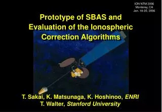
Evaluation by Prototype SBAS • Prototype SBAS software developed by ENRI (NTM 2006): • Computer software running on PC or UNIX; • Generates the complete 250-bit SBAS messages every seconds; • Simulates MSAS performance with user receiver simulator; • Available as an MSAS testbed; Measures benefit of additional monitor stations and evaluates new candidate algorithms. • Integration with the proposed algorithms: • Scenario of vertical ionospheric delay and GIVE is generated based on GEONET archive data with application of the proposed algorithms; • The prototype generated augmentation messages with ionospheric corrections induced as the scenario; • Tested for typical ionospheric condition (July 2004) and severe storm condition (October 2003).
User Protection • PPWAD Simulation • 03/10/29-31 • 3011 Tokyo • Condition: • Severe Storm • Algorithm: • Residual Bounding • (All GEONET sites) • Users are still protected by this algorithm during the severe storm.
System Availability PPWAD Simulation 04/7/22-24 Condition: Typical Ionosphere Algorithm: Residual Bounding (All GEONET sites) Contour plot for: APV-II Availability HAL = 40m VAL = 20m
Conclusion • Introduced new algorithms and usage of the external network to mitigate ionospheric threats: • Algorithms for bounding ionospheric corrections based on optimization of residual error measured by dense monitoring network; • Integration of GEONET as an external network. • Evaluation by prototype SBAS software: • Reduced GIVEI enables 100% availability of APV-II flight mode (VAL=20m) at most of Japanese airports; • No integrity failure (HMI condition). • Further investigations: • Consideration of threats against the proposed algorithms; • Reduction of the number of stations required for residual bounding; • Temporal variation and scintillation effects.
Announcement • Ionospheric delay database will be available shortly: • The datasets used in this study; and • Recent datasets generated daily from August 2007; • Each dataset is a file which consists of slant delays observed at all available GEONET stations with 300-second interval; Hardware biases of satellites and receivers are removed; • Access to URL: • http://www.enri.go.jp/sat/pro_eng.htm