Download
1 / 15
150 likes | 311 Views
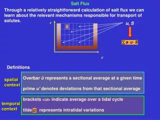
Salt Flux. Definitions Overbar ū represents a sectional average at a given time prime u’ denotes deviations from that sectional average brackets < u > indicate average over a tidal cycle tilde represents intratidal variations. spatial context. z. temporal context. y.

E N D
Salt Flux Definitions Overbar ū represents a sectional average at a given time prime u’ denotes deviations from that sectional average brackets <u> indicate average over a tidal cycle tilde represents intratidal variations spatial context z temporal context y Through a relatively straightforward calculation of salt flux we can learn about the relevant mechanisms responsible for transport of solutes. u, S a
Salt Flux Calculations The integral over the cross-section A of the product yields the rate of salt transport due to “mean flow” z = “shear dispersion” = “mean flow” y The salinity and axial velocity at any point (and at any given time) on a cross section of an estuary may each be represented as the sum of a cross-sectional average plus the deviation (in space) from that average: A The integral over the cross-section A of the product u’ S’ yields the instantaneous rate of salt transport due to “shear dispersion” The shear dispersion related to spatial variations through the water column is the vertical shear dispersion The shear dispersion related to variations across the width of the estuary is the transverse shear dispersion
z y Vertical Shear Dispersion x Horizontal Shear Dispersion x Shear Dispersion Shear Dispersion ~ Spatial covariance between u and S
Transport Calculation z, i Ai t Ai j area of each element y, j Make: ui= transverse mean at depth i ui t = transverse sum at depth i Ai t = area of transverse strip at depth i Water transport Qi j = Ai j ui j Salt transport Fi j = Ai j ui j Si j
z, i Ai t Ai j area of each element Av j y, j The transport through each transverse strip is then given by: Qi t = Ai t ui Fi t = Ai t ui Si Then make: uj= vertical or depth mean at strip j uv j = vertical sum of strip j Av j = area of vertical strip j Therefore, the transport through each vertical strip is given by: Qv j = Av j uj Fv j = Av j uj Sj And the rates of transport through the cross-section are represented as Q v t and F v t
z, i Ai t Ai j area of each element Av j y, j The vertical and transverse deviations of u i and u j are: u i’ = u i - ū u j’ = u j - ū ū is the sectional mean throughout A The “interaction” deviation is: u i j* = u i j - ( ū + u i’ + u j’ ) The rate of salt transport through the entire cross section is:
and using u i’ = u i - ū u j’ = u j - ū u i j* = u i j - ( ū + u i’ + u j’ ) Qi j = Ai j ui j Fi j = Ai j ui j Si j and That is the spatial representation at any given time. Now let’s look at time variations. We define a tidal oscillation as with zero average.
When including the temporal context to the Salt Flux calculation “tidal pumping” arises
Tidal pumping arises as the flood water mixes with relatively fresher water. A portion of that mixed water leaves the estuary on ebb. Then, fresher water leaves the estuary during ebb and saltier water enters the estuary during flood. This leads to down-estuary (seaward) pumping of fresher water, or equivalently, up-estuary pumping of salt. Tidal Pumping ~ Temporal covariance between u and S
Situation when Tidal pumping is most effective: time time flood flood Perfect covariance between and
The residual rate of transport of salt through the cross-section is: This relationship tells us the important mechanisms responsible for salt transport. The same relationship applies for sediment transport (e.g. Uncles et al, 1985, Estuaries, 8(3), 256-269). It has also been used for calculations of seston transport (Pino et al., 1994, ECSS, 38, 491-505). Most recent reference on the approach: Jay et al., 1997, Estuaries, 20(2), 262-280.
Strait of Magellan Seno Ballena Example of Salt Flux by Tidal Pumping
2 km Axial section typical depths > 200 m Seno Ballena Glacier
head 11 CTD stations along orange trajectory • hydrography suggests: • blocking of landward transport of salt by sill • - tidal pumping mouth
Total salt flux <uS> continuous line; Salt flux produced by mean flow <u><S> as dashed line; Tidal pumping salt flux <u’S’> as dotted line.