Download
1 / 29
340 likes | 753 Views
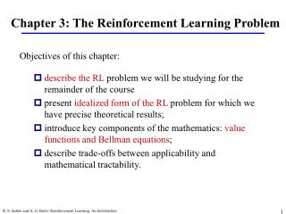
Chap. 13 Reinforcement Learning (RL). Machine Learning Tom M. Mitchell. outline. What is Reinforcement Learning? Methods Used in Reinforcement Learning Temporal Difference Methods Applications. Introduction. What ’ s reinforcement learning? History What reinforcement learning can do?

E N D
Chap. 13 Reinforcement Learning (RL) Machine Learning Tom M. Mitchell
outline • What is Reinforcement Learning? • Methods Used in Reinforcement Learning • Temporal Difference Methods • Applications
Introduction • What’s reinforcement learning? • History • What reinforcement learning can do? • Reinforcement Learning’s Element
What’s reinforcement Learning? Reinforcement learning address the question of how an autonomous agent that sense and acts in its environment can learn to choose optimal actions to achieve its goals. In Reinforcement learning , the computer is simply given a goal to achieve. The computer then learns how to achieve that goal by trial-and-error interactions with its environment.
What’s reinforcement Learning? • To provide the intuition behind reinforcement learning consider the problem of learning to ride a bicycle. • The goal given to the RL system is simply to ride the bicycle without falling over. • In the first trial, the RL system begins riding the bicycle and performs a series of actions that result in the bicycle being tilted 45 degrees to the right. At this point their are two actions possible: turn the handle bars left or turn them right.
What’s reinforcement Learning? • The RL system turns the handle bars to the left and immediately crashes to the ground, thus receiving a negative reinforcement. • The RL system has just learned not to turn the handle bars left when tilted 45 degrees to the right. • In the next trial The RL system knows not to turn the handle bars to the left, so it performs the only other possible action: turn right when tilted 45 degrees to the right.
What’s reinforcement Learning? • It immediately crashes to the ground, again receiving a strong negative reinforcement. • At this point the RL system has not only learned that turning the handle bars right or left when tilted 45 degrees to the right is bad, but that the "state" of being titled 45 degrees to the right is bad. • Again, the RL system begins another trial and performs a series of actions that result in the bicycle being tilted 40 degrees to the right. ……
What’s reinforcement Learning? • RL systems learn a mapping from situations to actions by trial-and-error interactions with a dynamic environment. The “goal” of the RL system is defined using the concept of a reward function, which is the exact function of future reinforcements(rewards) the agent seeks to maximize. • In other words, there exists a mapping from state/action pairs to reward; after performing an action in a given state the RL agent will receive some reward in the form of a scalar value. The RL agent learns to perform actions that will maximize the sum of the rewards received when starting from some initial state and proceeding to a terminal state. Agent State Reward environment a0 a1 a2 s0 s1 s2 r0 r2 r1 r0+ r1+ 2 r2+ … , where 0 < 1 The discount factor is used to exponentially decrease the weight of reinforcements received in the future
RL Vs. other function approximation • RL is similar in some respects to the function approximation problems discussed in other chapters. The target function to be learned in this case is a control policy : S -> A. A policydetermines which action should be performed in each state; a policy is a mapping from states to actions. • The valueof a state is defined as the sum of the rewardsreceived when starting in that state and following some fixed policy to a terminal state. • The optimal policy would therefore be the mapping from states to actions that maximizes the sum of the rewards when starting in an arbitrary state and performing actions until a terminal state is reached
RL Vs. other function approximation • This reinforcement learning problem differs from other function approximation tasks in several important respects. • Delayed reward: In RL, direct correspondence between the states and the actions is not available. The trainer provides only a sequence of immediate reward values as the agent executes its actions. Face the problem of temporal credit assignment. • Exploration: The agents influence the distribution of training examples by the action sequence it chooses. The question is which experimentation strategy produces most effective learning.
The Learning Task • Ways of formulation • Markov Decision Process (MDP) • Precise Task Definition • An Example
Ways of formulation • There are many ways to formulate the problem of learning sequential control strategies • Agent’s actions: Might be Deterministic or Nondeterministic • Agent may have or haven’t the ability of predicting the next state that will result from each action • Trainer of the agent: Expert(who shows it examples of optimal action sequences) or agent itself(train itself by performing actions of its own choice.)
States & Transitions s0 a1 a3 a2 s2 s1 s3 a7 a4 a5 a6 s5 s6 s7 s8
at at+1 at+2 st st+1 st+2 … rt rt+1 rt+2 Markov Decision Process. • Finite set of States : S; Set of Actions: A • t: discrete time step; • st: the state at time t; • at: the action at time t; • At each discrete time, agent observe states stS, and chooses action atA. • Then receive immediate reward: rt , And state change to: st+1 • Markov assumption:st+1= (st , at), rt=r (st , at) • i.e., rt, and st+1 depend only on current state and action • Functions and r may be nondeterministic • Functions and r not necessarily be known to agent
at at+1 at+2 st st+1 st+2 … rt rt+1 rt+2 Learning Task • Execute actions in the environment, observe results and • Learn a policy p : S A from states stS to actions atA that maximizes the accumulated reward : Vp(s) = rt+ rt+1+ 2 rt+2+… from any starting state st 0<<1 is the discount factor for future rewards. • Target function is p : S A • But there are no direct training examples of the form <s,a> • Training examples are of the form <<s,a>,r>
State Value Function • Consider deterministic environments, namely d(s,a) and r(s,a) are deterministic functions of s and a. • For each policy p: S A the agent might adopt, we define an evaluation function: Vp(s)= rt+ rt+1+ 2 rt+2+…= Si=0 rt+ii (13.1) where rt, rt+1,… are generated by following the policy p from start state s • Task: Learn the optimal policy p* that maximizes Vp(s) p* = argmaxp Vp(s) ,s (13.2)
Action Value Function • State value function denotes the reward for starting in state s and following policy p. Vp(s)= rt+ rt+1+ 2 rt+2+…= Si=0 rt+ii • Action value function denotes the reward for starting in state s, taking actiona and following policy p afterwards. Qp(s,a)= r(s,a) + rt+1+ 2 rt+2+… = r(s,a) + Vp (d(s,a))
Optimal Value Functions Concept of V* : V*(s) = maxp Vp(s) Concept of π*: The policy π which maximizes Vπ(s) for all states s. p*(s) = argmaxp Vp(s) ,s (13.2) π*(s)=argmaxa{r(s,a) + V*(d(s,a))} (13.3)
Example 0 0 100 0 G G 0 90 100 0 0 0 100 0 0 0 0 0 0 100 81 90 r(s, a) (immediate reward) values V*(s) values G G One Optimal policy all Optimal policies
hwk • 13.1 • 13.2
Example 73 100 90 100 66 66 R R 81 81 aright s1 s2 Q(s1, aright) r + maxa’Q (s2, a’ ) 0 + 0.9max{66,81,100} 90 0 0 0 0 90 100 G G 0 81 0 0 72 81 0 0 90 81 0 0 81 90 0 100 0 0 72 81 initial Q(s, a) values Q(s, a) values