Iterative Methods and Combinatorial Preconditioners
Iterative Methods and Combinatorial Preconditioners. Dignity. This talk is not about…. Credits.


Iterative Methods and Combinatorial Preconditioners
E N D
Presentation Transcript
Credits Finding effective support-tree preconditioners B. M. Maggs, G. L. Miller, O. Parekh, R. Ravi, and S. L. M. Woo. Proceedings of the 17th Annual ACM Symposium on Parallel Algorithms and Architectures (SPAA), July 2005. Combinatorial Preconditioners for Large, Sparse, Symmetric, Diagonally-Dominant Linear Systems Keith Gremban (CMU PhD 1996)
n by n matrix n by 1 vector known unknown known b A x = Linear Systems A useful way to do matrix algebra in your head: • Matrix-vector multiplication = Linear combination of matrix columns
0 1 0 1 0 1 0 1 0 1 1 1 1 2 1 3 1 1 1 2 1 3 a b b 2 1 2 2 2 3 2 1 2 2 2 3 + + a c = @ A @ A @ A @ A @ A 3 1 3 2 3 3 3 1 3 2 3 3 c 0 1 b 1 1 1 2 1 3 + + a c b 2 1 2 2 2 3 + + a c = @ A b 3 1 3 2 3 3 + + a c Matrix-Vector Multiplication • Using BTAT= (AB)T, (why do we need this, Maverick?)xTA should also be interpreted asa linear combination of the rows of A.
b A x = Strassen had a fastermethod to find A-1 How to Solve? • Find A-1 • Guess x repeatedly until we guess a solution • Gaussian Elimination
Circuit Voltage Problem Given a resistive network and the net current flow at each terminal, find the voltage at each node. 2A 2A A node with an external connection is a terminal. Otherwise it’s a junction. 3S 2S 1S Conductance is the reciprocal of resistance. It’s unit is siemens (S). 1S 4A
( ( ) ) ( ( ) ) 2 3 3 2 0 + ¡ ¡ + + ¡ ¡ v v v v v v v v = = 1 2 2 1 1 3 3 1 : ; Kirchoff’s Law of Current At each node, net current flow = 0. Consider v1. We have which after regrouping yields 2A 2A 3S v2 2S v1 v4 1S 1S I=VC 4A v3
Summing Up 2A 2A 3S v2 2S v1 v4 1S 1S 4A v3
Solving 2A 2A 3S 2S 2V 2V 3V 1S 1S 4A 0V
Did I say “LARGE”? • Imagine this being the power grid of America. 2A 2A 3S v2 2S v1 v4 1S 1S 4A v3
Laplacians Given a weighted, undirected graph G= (V, E), we can represent it as a Laplacian matrix. 3 v2 2 v1 v4 1 1 v3
Laplacians Laplacians have many interesting properties, such as • Diagonals ¸ 0 denotes total incident weights • Off-diagonals < 0 denotes individual edge weights • Row sum = 0 • Symmetric 3 v2 2 v1 v4 1 1 v3
Net Current Flow Lemma Suppose an n by n matrix A is the Laplacian of a resistive network G with n nodes. If y is the n-vector specifying the voltage at each node of G, then Ay is the n-vector representing the net current flow at each node.
Power Dissipation Lemma Suppose an n by n matrix A is the Laplacian of a resistive network G with n nodes. If y is the n-vector specifying the voltage at each node of G, then yTAy is the total power dissipated by G.
Sparsity Laplacians arising in practice are usually sparse. • The i-th row has (d+1) nonzeros if vi has d neighbors. 3 v2 2 v1 v4 1 1 v3
Sparse Matrix An n by n matrix is sparse when there are O(n) nonzeros. A reasonably-sized power grid has way more junctions and each junction has only a couple of neighbors. 3 v2 2 v1 v4 1 1 v3
Had Gauss owned a supercomputer… (Would he really work on Gaussian Elimination?)
1 R S 0 1 A Model Problem Let G(x,y) and g(x,y) be continuous functions defined in R and S respectively, where R and S are respectively the region and the boundary of the unit square (as in the figure).
2 2 @ @ ( ) ( ) u u u x y g x y = ( ) G + ; ; x y = ; 2 2 @ @ x y 1 R S If g(x,y) =0, this iscalled a Dirichletboundary condition. 0 1 A Model Problem We seek a function u(x,y) that satisfies Poisson’s equation in R and the boundary condition in S.
1 0 1 Discretization Imagine a uniform grid with a small spacing h. h
2 2 2 2 2 2 = = [ [ ( ( ) ) ( ( ) ) ( ( ) ) ] ] = = @ @ @ @ h h h h h h 2 2 + + + + ¡ ¡ ¡ ¡ u u y x u u x x y y u u x x y y u u x x y y s s ; ; ; ; ; ; ( ) ( ) ( ) h h 4 ¡ + ¡ ¡ u x y u x y u x y ; ; ; 2 ( ) ( ) ( ) h h h G ¡ + ¡ ¡ ¡ u x y u x y x y = ; ; ; Five-Point Difference Replace the partial derivatives by difference quotients The Poisson’s equation now becomes Exercise:Derive the 5-pt diff. eqt. from first principle (limit).
1 ( ( ) ) ( ( ) ) ( ( ) ) h h h h 4 4 ¡ ¡ + + ¡ ¡ ¡ ¡ 2 u u x x y y u u x x y y u u x x y y ( ) 1 ¡ ; ; ; ; ; ; h 2 2 ( ( ) ) ( ( ) ) ( ( ) ) h h h h h h G G ¡ ¡ + + ¡ ¡ ¡ ¡ ¡ ¡ u u x x y y u u x x y y x x y y = = ; ; ; ; ; ; For each point in R The total number of equations is . Now write them in the matrix form, we’ve got one BIG linear system to solve!
( ) ( ( ( ) ) ) ( ( ) ) ( ( ( ) ) ) h h 4 4 4 3 3 1 1 2 4 1 1 3 2 2 1 ¡ + ¡ ¡ ¡ ¡ ¡ ¡ u x y u u u x y u u u x u u y ; ; ; ; ; ; ; ; ; ( ( ) ) ( ( ) ) ( ( ) ) 2 G G 3 2 3 1 3 0 4 1 3 3 1 0 ( ) ( ) ( ) ¡ ¡ ¡ + + ¡ h h h G ¡ + ¡ ¡ ¡ u u u u = = u x y u x y x y = ; ; ; ; ; ; ; ; ; An Example Consider u3,1, we have which can be rearranged to 4 u32 u21 u31 u41 u30 0 4
( ) ( ) ( ) h h 4 ¡ + ¡ ¡ u x y u x y u x y ; ; ; 2 ( ) ( ) ( ) h h h G ¡ + ¡ ¡ ¡ u x y u x y x y = ; ; ; An Example Each row and column can have a maximum of 5 nonzeros.
Sparse Matrix Again Really, it’s rare to see large dense matrices arising from applications.
Laplacian??? I showed you a system that is not quite Laplacian. • We’ve got way too many boundary points in a 3x3 example.
Making It Laplacian We add a dummy variable and force it to zero.(How to force? Well, look at the rank of this matrix first…)
Sparse Matrix Representation A simple scheme • An array of columns, where each column Aj is a linked-list of tuples (i,x).
Solving Sparse Systems Gaussian Elimination again? Let’s look at one elimination step.
Solving Sparse Systems Gaussian Elimination introduces fill.
Solving Sparse Systems Gaussian Elimination introduces fill.
Fill Of course it depends on the elimination order. • Finding an elimination order with minimal fill is hopelessGarey and Johnson-GT46, Yannakakis SIAM JADM 1981 • O(logn) ApproximationSudipto Guha, FOCS 2000Nested Graph Dissection and Approximation Algorithms • (nlogn) lower bound on fill(Maverick still has not dug up the paper…)
b A x = When Fill Matters… • Find A-1 • Guess x repeatedly until we guessed a solution • Gaussian Elimination
Inverse Of Sparse Matrices …are not necessarily sparse either! BB-1
b A x = And the winner is… • Find A-1 • Guess x repeatedly until we guessed a solution • Gaussian Elimination Can we be so lucky?
Iterative Methods Checkpoint • How large linear system actually arise in practice • Why Gaussian Elimination may not be the way to go
The Basic Idea Start off with a guess x (0). Use x (i ) to compute x (i+1) until convergence. We hope • the process converges in a small number of iterations • each iteration is efficient
Domain Range Residual x ( ) ( ) ( ) i i i 1 + ( ) b A ¡ ¡ x x x = b x(i+1) Ax(i) x(i) The RF Method [Richardson, 1910] A Test Correct
x ( ) ( ) ( ) i i i 1 + ( ) b A ¡ ¡ x x x = b x(i+1) Ax(i) x(i) Why should it converge at all? Domain Range Test Correct
( ) G 1 < ( ) ( ) i i 1 + ½ k G + . x x = ( ) ( ) ( ) i i i 1 + ( ) b A ¡ ¡ x x x = It only converges when… Theorem A first-order stationary iterative method converges iff (A) is the maximumabsolute eigenvalue of A
b A x = Fate? Once we are given the system, we do not have any control on A and b. • How do we guarantee even convergence?
1 1 b B A B - - x = Preconditioning Instead of dealing with A and b,we now deal with B-1A and B-1b. The word “preconditioning”originated with Turing in 1948,but his idea was slightly different.
( ) ( ) ( ) i i i 1 1 1 + ( ) b B A B - - ¡ ¡ x x x = Preconditioned RF Since we may precompute B-1b by solving By=b, each iteration is dominated by computing B-1Ax(i), which is • a multiplication step Ax(i) and • a direct-solve step Bz=Ax(i). Hence a preconditioned iterative method is in fact a hybrid.
I A Trivial What’s the point? The Art of Preconditioning We have a lot of flexibility in choosing B. • Solving Bz=Ax(i) must be fast • B should approximate A well for a low iteration count B
( ) ( ) ( ) i i i 1 1 1 + ( ) b B A B - - ¡ ¡ x x x = Classics Jacobi • Let D be the diagonal sub-matrix of A.Pick B=D. Gauss-Seidel • Let L be the lower triangular part of A w/ zero diagonalsPick B=L+D.
“Combinatorial” We choose to measure how well B approximates Aby comparing combinatorial properties of (the graphs represented by) A and B. • Hence the term “Combinatorial Preconditioner”.