Download
1 / 35
350 likes | 462 Views
Explore the velocity and scalar fields in a complex reactor setup using advanced experimental methods. Understand turbulent mixing dynamics for applications in combustion, propulsion, and industrial processes.

E N D
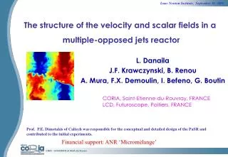
The structure of the velocity and scalar fields in a multiple-opposed jets reactor L. Danaila J.F. Krawczynski, B. Renou A. Mura, F.X. Demoulin, I. Befeno, G. Boutin CORIA, Saint-Etienne-du-Rouvray, FRANCE LCD, Futuroscope, Poitiers, FRANCE Prof. P.E. Dimotakis of Caltech was responsible for the conceptual and detailed design of the PaSR and contributed to the initial experiments. Financial support: ANR ‘Micromélange’
OUTLINE I. Motivation of the great work: theoretical vs. applied research II. Experimental set-up: Partially Stirred Reactor (PaSR) Experimental methods: PIV, LDV (1 and 2 points), PLIF III. Description of the flow Instantaneous aspect: instabilities in the central region Mean velocity field Fluctuating field and isotropy Spectral analysis Fine-scale properties of the flow IV. Characterization of the mixing V. Conclusions
Why? Combustion, propulsion, chemical and other industrial problems How? Create SHI – Stationary, (nearly) Homogeneous, and (nearly) Isotropic flow and mixing:closed vessels and/or propellers, HEV… The ‘porcupine’: R. Betchov, 1957 ‘ Synthetic jets’ in cubic chamber - W. Hwang and J.K. Eaton (E. Fluids, 2003) Propellers - Birouk, Sahr and Gokalp (F. Turb. & Comb, 2003) Synthetic jets - J.P. Marié French Washing Machine Ignition, stability, extinction ? Pollutants emissions ? Better efficiency ? I. MOTIVATION: Improved understanding of Turbulent Mixing
Z0 Z1 Z0 Z1 Exit I. MOTIVATION: Improved understanding of Turbulent Mixing • Issues? • Optimal configuration: basic PaSR (Partially Stirred Reactor) model S.M. Correa and M.E. Braaten (1993) Assumptions: Mean: Homogeneity at large scales, Stationary case Fluctuations of the smaller scales Main advantages: Ideal tool to test micro-mixing models (IEM, Curl, Curl modified, …) Characteristic times: tR (Residence time); tT (Turbulence time); tM (Mixing time); tC (Chemical time)
I. MOTIVATION: Improved understanding of Turbulent Mixing • Question • Why a SHI flow must be created since few such flows exist in reality ? • Turbulent flows are very complex by nature interest to examine simpler flows • Create a reference and an academic experimental configuration • Ideal to develop and valid statistical theories of turbulence Analytical approaches • Limitation of DNS for high Rel High Rel can be reached in forced turbulence Ultra Low-NOx Combustion Dynamics
II. EXPERIMENTAL SET-UP • Design of the PaSR versus objectives: • Large range of Reynolds number Rel: 60 – 1000 • Pressure variations 1- 3 bars • Different flow configurations • Pairs of Impinging jets • Sheared flow • Modularity of the system • Large range of flow rates and internal volumes • Characteristic times tRandtT compatible with chemical time • Reactive configuration for future work P. Paranthoen, R. Borghi and M. Mouquallid (1991)
II. EXPERIMENTAL SET-UP* • Volume PaSR: V = 11116 cm3 • Injection velocity: UJ = 4.5 - 47 m/s • Return flow= porous top/bottom plates • Residence time: tR = 8 -46 ms Reynolds number 60 Rl 1000 (center) *Prof. P.E. Dimotakis of Caltech was responsible for the conceptual and detailed design of the PaSR and contributed to the initial experiments.
II. EXPERIMENTAL SET-UP and measurements Velocity field: 1) Particle velocimetry • Resolution and noise limitations • PIV resolution linked to size of interrogation/correlation window, e.g., 16, 32, and 64 pix2, and processing algorithm choices • Does not resolve small scales: the smallest 100% =1.7 mm • Problem to estimate energy dissipation directly • Towards adaptive/optimal vector processing/filtering 2) LDV in (1 point and) 2 points • Simultaneous measurements of One velocity component in two points of the space: spatial resolution 200 * 50 microns; sampling frequency= 20 kHZ Scalar field: PLIF on acetone Small-scale limitations set by spatial resolution (pixel/laser-sheet size) The smallest resolved scale 100% =0.7 mm Signal-to-noise ratio per pixel • Adaptive/optimal image processing/filtering
26252 8 injection conditions 6089 II. EXPERIMENTAL SET-UP and measurements Re 104 2 Geometries: H/D=3 H/D=5
z y x III. DESCRIPTION of the FLOW: Mean flow properties A forced box turbulence -locally, in each part of the PaSR, we recognize a ‘classical’ zone, e.g. Injection zone = impinging jets « Mixing » zone = stagnation zone Return flow (top/bottom porous) Presence ofgiant vorticity rings =16 French Washing machines
III. DESCRIPTION of the FLOW: Mean flow properties Strong circomferential mixing layers GIANT COHERENT RINGS
2 3 z y Strong energy injection 1 l x III. DESCRIPTION of the FLOW: fluctuating field
III. DESCRIPTION of the FLOW: fluctuating field Energy Isotropy? II I Structures: azimuthal enstrophy
III. DESCRIPTION of the FLOW: fluctuating field; spectral approach from PIV • Horizontal and vertical cut in 2D spectrum • Energy injection • Restricted scaling range E(k) k-5/3 • Scaling range E(k) k-3 1D spectra in • k-2.33 • Properties similar to turbulence in rotation presence of coherent structures CUT-OFF k-3 Energy injection What about the small scales? Unresolved by PIV Large-scale information from PIV LDV measurements in 1 and 2 points.
Vinj=7m/s III. DESCRIPTION of the FLOW: fluctuating field; local approach Vinj=17m/s II II I I I : Impinging point II: Return zone (Gaussian) From LES, vortices (Q criterium) Local approach
3-rd order SF 2-nd order SF with the Kolmogorov constant Ck=2 .. Normalized dissipation which L? Attention to initial conditions versus universality .. However, a reliable test The most reliable test is the 1—point energy budget equation, when the pressure-related terms could be neglected (point II). III. DESCRIPTION of the FLOW: fluctuating field; local approach; PIV for determining small-scale properties ‘Traditional’ Spectral method Inertial range Corrected spectra (see Lavoie et al. 2007); Drawback: the theoretical 3D spectrum E(k) should be known .. Drawback: spectra are to be calculated over locally homogeneous regions of the flow, and require 2^N points Here:
III. DESCRIPTION of the FLOW: fluctuating field; PIV for determining small scale properties 3-rd order SF • Iterative Methodology • Measure , consider the Kolmogorov constant as 4/5 and infer Epsilon • Determine the turbulent Reynolds number, infer the Kolmogorov constant (forced turbulence) and start again Grid turbulence data: Mydlarski & Warhaft 1996, Danaila et al. 1999
III. DESCRIPTION of the FLOW: fluctuating field; PIV for determining small scale properties 3-rd order SF JETS Antonia & Burattini, JFM 2006
The other tests 2-rd order SF with the Kolmogorov constant Normalized dissipation which L? Attention to initial conditions versus universality .. However, a reliable test for The most reliable test is the 1—point energy budget equation, when the pressure-related terms might be neglected (point II). III. DESCRIPTION of the FLOW: fluctuating field; PIV for determining small scale properties
III. DESCRIPTION of the FLOW: fluctuating field; back to PIV for determining small scale properties For the stagnation point I, The pressure-velocity correlation Term cannot be neglected, since The mean pressure is important At high Reynolds and low ratios H/D
III. DESCRIPTION of the FLOW: fluctuating field; back to PIV for determining small scale properties RESULTS: Point I PIV 3 other methods PIV finite differences
III. DESCRIPTION of the FLOW: fluctuating field; back to PIV for determining small scale properties RESULTS: Point I Conclusion (point I) R_lambda maximum=750
III. DESCRIPTION of the FLOW: fluctuating field; back to PIV for determining small scale properties RESULTS: Point II PIV 4 other methods PIV finite differences
III. DESCRIPTION of the FLOW: fluctuating field; back to PIV for determining small scale properties RESULTS: Point II Conclusion (point II) R_lambda maximum=350
Residence time Cascade time Kolmogorov time Red circles: point I Blue diamonds: point II
a) LDV in 1 point mean velocity, RMS, small-scales quantities (definitions, correlations, SF2, SF3, 1-point energy budget equation… ). Good to determine the RMS and to compare with the PIV results (15% difference). Drawback: Taylor’s hypothesis is needed, in a flow where the turbulence intensity varies from 100% to infinity (stagnation points ..). LDV in two points simultaneous measurements of one velocity component in 2 spatial points (separation parallel to the measured velocity direction)… many points. Different methods: SF2, SF3, definition of 1-point energy budget equation (pressure … good for point II). III. DESCRIPTION of the FLOW: fluctuating field; LDV for determining small scale properties These measurements only reinforce the Conclusions pointed out by large-scale PIV
Interface probability, along the jets axis l IV. DESCRIPTION of the scalar mixing: fluctuating field z = 1 z = 0 • Jets instabilities (Denshchikov et al. 1978) Gaussian shape of the Pdf
IV. Description of the scalar mixing: fluctuating field Instantaneous fields of the mixing fraction z H/D=3 H/D=5 Large pannel of structures Large-scale instabilities (jets flutter) Mechanisms controlling the mixing?
H/D=3 H/D=5 Invariance / injection conditions Similarity IV. Description of the scalar mixing: mean field
Conclusions • Pairs of impinging jets • Return flow by top/bottom porous locally axisymmetric flow • strong sheared layers • Flow only (very) locally homogeneous difficulties to apply the classical spectral approach (spectral corrections because of finite size of the probe, and so on ..) • Techniques to infer the (local) dissipation and turbulent Reynolds number • Structure functions (SF2, SF3) are better adapted • Inertial-range properties are quite useful to infer small-scale properties of the flow (dissipation) • 1-point energy budget equation- where the pressure velocity correlations are negligible
Conclusions • The turbulent Reynolds number goes up to • 750 in the points among opposed jets • 350 in the return flow (Gaussian statistics) • Mixing is done more rapidly than the velocity field: one injection • point, and at one very small scale • The velocity field is injected at several scales and in several points • Analogy kinetic energy- scalar does not hold
IV. Description of the scalar mixing: fluctuating field Influence des grandes structures de concentration uniforme Evolution du pic vers des niveaux de concentration inférieure présence de structures à petites échelles Plus grande stabilité gradients plus importants mélange aux petites échelles plus efficace
III. Description of the flow: fluctuating field; PIV for determining small scale properties 3-rd order SF MID-SPAN JETS The sign changes at Large scales (inhomogeneity)
Results IV. Description of the scalar mixing: fluctuating field • Champ instantané de la vitesse azimutale dans le plan des jets expérience simulation