Download
1 / 30
300 likes | 515 Views
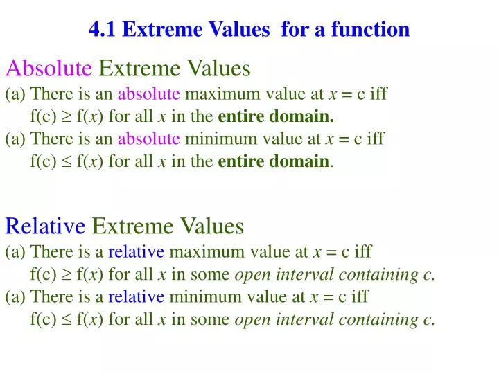
4.1 Extreme Values for a function. Absolute Extreme Values There is an absolute maximum value at x = c iff f(c) f( x ) for all x in the entire domain. There is an absolute minimum value at x = c iff f(c) f( x ) for all x in the entire domain .

E N D
4.1 Extreme Values for a function • Absolute Extreme Values • There is an absolute maximum value at x = c iff • f(c) f(x) for all x in the entire domain. • There is an absolute minimum value at x = c iff • f(c) f(x) for all x in the entire domain. • Relative Extreme Values • There is a relative maximum value at x = c iff • f(c) f(x) for all x in some open interval containing c. • There is a relative minimum value at x = c iff • f(c) f(x) for all x in some open interval containing c.
Locations of Extreme values If f(x) has a maximum or minimum value at x = c it must occur at one of the following locations: • Where f (c) =0 • Where f (c ) is undefined • At an endpoint of a closed interval **Values in the domain of f where f (c) is zero or is undefined are called critical values of the function.***
Maxima and Minima on closed interval for continuous function must exist.
Local Max A curve with a local maximum value. The slope at c, is zero.
4.3 First Derivative test for Increasing and Decreasing functions • If a function is continuous on [a, b] and differentiable on (a,b) • If f > 0 at each point of (a,b) then f increases on [a,b]. • If f < 0 at each point of (a,b) then f decreases on [a,b].
Find the critical points and identify intervals on which f is increasing and decreasing.
First derivative test for Local Extrema At a critical point x = c • f has a local minimum iff changes from negative to positive at c. • f has a local maximum iff changes from positive to negative at c. • There is no extreme value if the sign of f does not change. Could be a horizontal tangent without direction change.
Concavity Figure 3.24: The graph of f (x) = x3 is concave down on (–, 0) and concave up on (0, ).
Second derivative test for Concavity A graph is concave up on any interval where The second derivative is positive. A graph is concave down on any interval where The second derivative is negative. A point of inflection for a function Occurs where the concavity changes
Second derivative test for extreme values - - - + + + If there is a critical value at x = c and conclusion A local max at x = c A local min at x = c inconclusive
Section 4.3 · Figures 11 Graph of the curve Section 1 / Figure 1 A © 2003 Brooks/Cole, a division of Thomson Learning, Inc. Thomson Learning™ is a trademark used herein under license.
Finding intervals of concave up and concave down and Inflection points The graph of f (x) = x4 – 4x3 + 10.
4. 4 Limits to Infinity (End behavior) Figure 1.42: The blue graph of f (x) = x + e–x looks like the graph of g(x) = x (black) to the right of the y-axis and like the graph of h(x) = e–x (red) to the left of the y-axis. (Example 1) What happens to the value of the function when the value of x increases without bound? What happens to the value of the function when the value of x decreases without bound?
Figure 1.27: The function in Example 3. Divide each term by highest power of x in the denominator and calculate limits As x gets larger and larger, the function gets closer and closer to 5/3.
Figure 1.27: The function in Example 3. Divide each term by highest power of x in the denominator and calculate limits As x gets larger and larger, the function gets closer and closer to 0.
Figure 1.27: The function in Example 3. Divide each term by highest power of x in the denominator and calculate limits As x gets larger and larger, the function decreases without bound.
Figure 1.27: The function in Example 3. As x gets larger and larger, the function gets closer and closer to 5/3. When the limit to infinity exists, at y = L we can say that the line y = L is a horizontal asymptote.
Horizontal Asymptote Figure 1.27: The function in Example 3.
Limits that are infinite (y increases without bound) An infinite limit will exist as x approaches a finite value when direct substituion produces If an infinite limit occurs at x = c we have a vertical asymptote with the equation x = c.
Slant Asymptote As x gets larger and larger, the graph gets closer and closer to the line Figure 1.29: The function in Example 5(a). As x gets smaller and smaller, the graph gets closer to the same line. You can use long division to rewrite the given function. There is a vertical asymptote at x = - 4 / 7
4.6Different scales Graphs of the polynomial Section 1 / Figure 1 © 2003 Brooks/Cole, a division of Thomson Learning, Inc. Thomson Learning™ is a trademark used herein under license.
Graphs of derivatives Derivatives of the polynomial Section 1 / Figure 1 © 2003 Brooks/Cole, a division of Thomson Learning, Inc. Thomson Learning™ is a trademark used herein under license.
Section 4.6 · Figures 19, 20 The family of functions Section 1 / Figure 1