Markov Chain Part 1
210 likes | 592 Views
Markov Chain Part 1. 多媒體系統研究群 指導老師:林朝興 博士 學生:鄭義繼. Outline. Stochastic Process Markov Chain. Stochastic Process. A stochastic process is a indexed collection of random variables {X t } = { X 0 , X 1 , X 2 , … } for describing the behavior of a system operating over some period of time.

Markov Chain Part 1
E N D
Presentation Transcript
Markov Chain Part 1 多媒體系統研究群 指導老師:林朝興 博士 學生:鄭義繼
Outline • Stochastic Process • Markov Chain
Stochastic Process • A stochastic process is a indexed collection of random variables {Xt} = { X0, X1, X2, … } for describing the behavior of a system operating over some period of time. • For example : • X0 = 3, X1 = 2, X2 = 1, X3 = 0, X4 = 3, X5 = 1
Stochastic Process (cont.) • An inventory example: • A camera store stocks a particular model camera. • Dt represents the demand for this camera during week t. • Dt has a Poisson distribution with a mean of 1. • Xt represents the number of cameras on hand at the end of week t. ( X0 = 3 ) • If there are no cameras in stock on Saturday night, the store orders three cameras. • { Xt } is a stochastic process. • Xt+1 = max{ 3 – Dt+1, 0 } if Xt = 0 max{ Xt - Dt+1, 0 } if Xt≥ 0
Markov Chain • A stochastic process {Xt} is a Markov chain if it has Markovian property. • Markovian property: • P{ Xt+1 = j | X0 = k0, X1 = k1, ..., Xt-1 = kt-1, Xt = i } = P{ Xt+1 = j | Xt = i } • P{ Xt+1 = j | Xt = i } is called the transition probability.
Markov Chain (con.) • Stationary transition probability: • If ,for each i and j, P{ Xt+1 = j | Xt = i } = P{ X1 = j | X0 = i }, for all t, then the transition probability are said to be stationary.
state 0 1 2 3 0 p00 p01 p02 p03 1 P = p10 p11 p12 p13 2 3 p20 p21 p22 p23 p30 p31 p32 p33 Markov Chain (con.) • Formulating the inventory example: • Transition matrix:
state 0 1 2 3 0 0.080 0.184 0.368 0.368 1 P = 0.632 0.368 0.000 0.000 2 3 0.264 0.368 0.368 0.000 0.080 0.184 0.368 0.368 Markov Chain (con.) • Xt+1 = max{ 3 – Dt+1, 0 } if Xt = 0 max{ Xt - Dt+1, 0 } if Xt≥ 1 • p03 = P{ Dt+1 = 0 } = 0.368 • p02 = P{ Dt+1 = 1 } = 0.368 • p01 = P{ Dt+1 = 2 } = 0.184 • p00 = P{ Dt+1≥ 3 } = 0.080
Markov Chain (con.) • The state transition diagram:
state 0 1 ... M 0 P00(n) P01(n) P0M(n) ... 1 P(n)= . . P10(n) P11(n) P1M(n) ... M ... ... ... ... PM0(n) PM1(n) PMM(n) ... Markov Chain (con.) • n-step transition probability : • pij(n) = P{ Xt+n = j | Xt = i } • n-step transition matrix :
Markov Chain (con.) • Chapman-Kolmogorove Equation : • The special cases of m = 1 leads to : • Thus the n-step transition probability can be obtained from one-step transition probability recursively. for all i = 0, 1, …, M, j = 0, 1, …, M, and any m = 1, 2, …, n-1, n = m+1, m+2, … for all i and j
state state 0 0 1 1 2 2 3 3 0 0 0.289 0.080 0.286 0.184 0.261 0.368 0.368 0.164 1 1 P(4)= P = 0.632 0.282 0.368 0.285 0.000 0.268 0.166 0.000 2 2 3 3 0.284 0.264 0.283 0.368 0.368 0.263 0.171 0.000 0.289 0.080 0.286 0.184 0.368 0.261 0.368 0.164 Markov Chain (con.) • Conclusion : • P(n) = PP(n-1) = PPP(n-2) = ... = Pn • n-step transition matrix for the inventory example :
Markov Chain (con.) • What is the probability that the camera store will have three cameras on hand 4 weeks after the inventory system began ? • P{ Xn = j } = P{ X0 = 0 }p0j(n) + P{ X0 = 1 } p1j(n) + ... + P{ X0 = M } pMj(n) • P{ X4 = 3 } = P{ X0 = 0 }p03(4) + P{ X0 = 1 } p13(4) + P{ X0 = 2 } p23(4) + P{ X0 = 3 } p33(4) = (1) p33(4) = 0.164
state state 0 0 1 1 2 2 3 3 0 0 0.080 0.286 0.184 0.285 0.368 0.264 0.166 0.368 1 1 P = P(8)= 0.286 0.632 0.285 0.368 0.264 0.000 0.000 0.166 2 2 3 3 0.264 0.286 0.368 0.285 0.264 0.368 0.000 0.166 0.080 0.286 0.184 0.285 0.264 0.368 0.166 0.368 Markov Chain (con.) • Long-Run Properties of Markov Chain • Steady-State Probability
state 0 1 2 3 0 p0 p1 p2 p3 1 p0 p1 p2 p3 2 3 p0 p1 p2 p3 p0 p1 p2 p3 Markov Chain (con.) • The steady-state probability implies that there is a limiting probability that the system will be in each state j after a large number of transitions, and that this probability is independent of the initial state. • Not all Markov chains have this property.
for i = 0, 1, …, M Markov Chain (con.) • Steady-State Equations : • , which consists of M+2 equations in M+1 unknowns.
Markov Chain (con.) • The inventory example : • p0 = p0p00 + p1p10 + p2p20 + p3p30 , • p1 = p0p01 + p1p11 + p2p21 + p3p31 , • p2 = p0p02 + p1p12 + p2p22 + p3p32 , • p3 = p0p03 + p1p13 + p2p23 + p3p33 , • 1 = p0 + p1 + p2 + p3. • p0 = 0.080p0 + o.632p1 + 0.264p2 + 0.080p3 , • p1 = 0.184p0 + 0.368p1 + 0.368p2 + 0.184p3 , • p2 = 0.368p0 + + 0.368p2 + 0.368p3 , • p3 = 0.368p0 + + + 0.368p3 , • 1 = p0 + p1 + p2 + p3. • p0 = 0.286, p1 = 0.285, p2 = 0.263, p3 = 0.166
Reference • Hillier and Lieberman, “Introduction to Operations Research”, seventh edition, McGraw Hill