Download

1 / 56
580 likes | 802 Views
Clustering and Classification – Introduction to Machine Learning BMI 730 . Kun Huang Department of Biomedical Informatics Ohio State University. How do we use microarray? Profiling Clustering. Cluster to detect gene clusters and regulatory networks. Cluster to detect patient subgroups.

E N D
Clustering and Classification – Introduction to Machine LearningBMI 730 Kun Huang Department of Biomedical Informatics Ohio State University
How do we use microarray? • Profiling • Clustering Cluster to detect gene clusters and regulatory networks Cluster to detect patient subgroups
Clustering and Classification • Preprocessing • Distance measures • Popular algorithms (not necessarily the best ones) • More sophisticated ones • Evaluation • Data mining
Clustering or classification? • Is training data available? • What domain specific knowledge can be applied? • What preprocessing of data is needed? • Log / data scale and numerical stability • Filtering / denoising • Nonlinear kernel • Feature selection (do I need to use all the data?) • Is the dimensionality of the data too high?
How do we process microarray data (clustering)? • Feature selection – genes, transformations of expression levels. • Genes discovered in the class comparison (t-test). Risk: missing genes. • Iterative approach : select genes under different p-value cutoff, then select the one with good performance using cross-validation. • Principal components (pro and con). • Discriminant analysis (e.g., LDA).
Dimensionality Reduction • Principal component analysis (PCA) • Singular value decomposition (SVD) • Karhunen-Loevetransform (KLT) Basis for P SVD
Principal Component Analysis (PCA) - Other things to consider • Numerical balance/data normalization • Noisy direction • Continuous vs. discrete data • Principal components are orthogonal to each other, however, biological data are not • Principal components are linear combinations of original data • Prior knowledge is important • PCA is not clustering!
B 2.0 1.5 1.0 0.5 . . . . . . . . . . . . . . . w A 0.5 1.0 1.5 2.0 Dimensionality reduction: linear discriminant analysis (LDA) (From S. Wu’s website)
B 2.0 1.5 1.0 0.5 . . . . . . . . . A . . . . 0.5 1.0 1.5 2.0 . . w Linear Discriminant Analysis (From S. Wu’s website)
Visualization of Microarray Data • Multidimensional scaling (MDS) • High-dimensional coordinates unknown • Distances between the points are known • The distance may not be Euclidean, but the embedding maintains the distance in a Euclidean space • Try different dimensions (from one to ???) • At each dimension, perform optimal embedding to minimize embedding error • Plot embedding error (residue) vs. dimension • Pick the knee point
Visualization of Microarray Data Multidimensional scaling (MDS)
Clustering and Classification • Preprocessing • Distance measures • Popular algorithms (not necessarily the best ones) • More sophisticated ones • Evaluation • Data mining
Distance Measure (Metric?) • What do you mean by “similar”? • Euclidean • Uncentered correlation • Pearson correlation
Distance Metric • Euclidean 102123_at Lip1 1596.000 2040.900 1277.000 4090.500 1357.600 1039.200 1387.300 3189.000 1321.300 2164.400 868.600 185.300 266.400 2527.800 160552_at Ap1s1 4144.400 3986.900 3083.100 6105.900 3245.800 4468.400 7295.000 5410.900 3162.100 4100.900 4603.200 6066.200 5505.800 5702.700 dE(Lip1, Ap1s1) = 12883
Distance Metric • Pearson Correlation 102123_at Lip1 1596.000 2040.900 1277.000 4090.500 1357.600 1039.200 1387.300 3189.000 1321.300 2164.400 868.600 185.300 266.400 2527.800 160552_at Ap1s1 4144.400 3986.900 3083.100 6105.900 3245.800 4468.400 7295.000 5410.900 3162.100 4100.900 4603.200 6066.200 5505.800 5702.700 dP(Lip1, Ap1s1) = 0.904
Distance Metric • Pearson Correlation Ranges from 1 to -1. r = 1 r = -1
Distance Metric • Uncentered Correlation 102123_at Lip1 1596.000 2040.900 1277.000 4090.500 1357.600 1039.200 1387.300 3189.000 1321.300 2164.400 868.600 185.300 266.400 2527.800 160552_at Ap1s1 4144.400 3986.900 3083.100 6105.900 3245.800 4468.400 7295.000 5410.900 3162.100 4100.900 4603.200 6066.200 5505.800 5702.700 du(Lip1, Ap1s1) = 0.835 q About 33.4o
Distance Metric • Difference between Pearson correlation and uncentered correlation 102123_at Lip1 1596.000 2040.900 1277.000 4090.500 1357.600 1039.200 1387.300 3189.000 1321.300 2164.400 868.600 185.300 266.400 2527.800 160552_at Ap1s1 4144.400 3986.900 3083.100 6105.900 3245.800 4468.400 7295.000 5410.900 3162.100 4100.900 4603.200 6066.200 5505.800 5702.700 Uncentered correlation All are considered signals Pearson correlation Baseline expression possible
Distance Metric • Difference between Euclidean and correlation
Distance Metric • Missing: negative correlation may also mean “close” in signal pathway (1-|PCC|, 1-PCC^2)
Clustering and Classification • Preprocessing • Distance measures • Popular algorithms (not necessarily the best ones) • More sophisticated ones • Evaluation • Data mining
How do we process microarray data (clustering)? • Unsupervised Learning – Hierarchical Clustering
How do we process microarray data (clustering)? • Unsupervised Learning – Hierarchical Clustering Single linkage: The linking distance is the minimum distance between two clusters.
How do we process microarray data (clustering)? • Unsupervised Learning – Hierarchical Clustering Complete linkage: The linking distance is the maximum distance between two clusters.
How do we process microarray data (clustering)? • Unsupervised Learning – Hierarchical Clustering • Average linkage/UPGMA: The linking distance is the average of all pair-wise distances between members of the two clusters. Since all genes and samples carry equal weight, the linkage is an Unweighted Pair Group Method with Arithmetic Means (UPGMA).
How do we process microarray data (clustering)? • Unsupervised Learning – Hierarchical Clustering • Single linkage – Prone to chaining and sensitive to noise • Complete linkage – Tends to produce compact clusters • Average linkage – Sensitive to distance metric
Unsupervised Learning – Hierarchical Clustering • Dendrograms • Distance – the height each horizontal line represents the distance between the two groups it merges. • Order – Opensource R uses the convention that the tighter clusters are on the left. Others proposed to use expression values, loci on chromosomes, and other ranking criteria.
Unsupervised Learning - K-means • Vector quantization • K-D trees • Need to try different K, sensitive to initialization
Unsupervised Learning - K-means [cidx, ctrs] = kmeans(yeastvalueshighexp, 4, 'dist', 'corr', 'rep',20); Metric K
Unsupervised Learning - K-means • Number of class K needs to be specified • Does not always converge • Sensitive to initialization
Unsupervised Learning • Self-organized maps (SOM) • Neural network based method • Originally used as a visualization method for visualize (embedding) high-dimensional data • Also related vector quantization • The idea is to map close data points to the same discrete level
Issues • Lack of consistency or representative features (5.3 TP53 + 0.8 PTEN doesn’t make sense) • Data structure is missing • Not robust to outliers and noise D’Haeseleer 2005 Nat. Biotechnol 23(12):1499-501
Review of Microarray and Gene Discovery • Clustering and Classification • Preprocessing • Distance measures • Popular algorithms (not necessarily the best ones) • More sophisticated ones • Evaluation • Data mining
Model-based clustering methods (Han) http://www.cs.umd.edu/~bhhan/research2.html Pan et al. Genome Biology 2002 3:research0009.1 doi:10.1186/gb-2002-3-2-research0009
Supervised Learning • Support vector machines (SVM) and Kernels • Only (binary) classifier, no data model
Supervised Learning - Support vector machines (SVM) and Kernels • Kernel – nonlinear mapping
Prior prob. Conditional prob. • Supervised Learning - Naïve Bayesian classifier • Bayes rule • Maximum a posterior (MAP)
Review of Microarray and Gene Discovery • Clustering and Classification • Preprocessing • Distance measures • Popular algorithms (not necessarily the best ones) • More sophisticated ones • Evaluation • Data mining
Testing sample Prediction error Training sample Model complexity (reproduced from Hastie et.al.) • Accuracy vs. generality • Overfitting • Model selection
Assessing the Validity of Clusters • Most clustering algorithms do not assume any structure or a prior relationship among the genes. However, the found clusters should more or less reflect the structures (e.g., pathways). (An interesting research problem is to develop new algorithms that can accommodate such relationships.) • If different patients are grouped into clusters, it implies that there are subtypes for the disease, which is a big claim and must be validated using other methods (e.g., pathology). • Relationship with external variables is important. E.g., clustering on cells from different tissue types may correspond to the relationship among the tissues.
Assessing the Validity of Clusters • Where should we cut the dendrograms? • Which clustering results should we believe, i.e., different (or even the same) clustering algorithms may find different clustering results? • Many tests are flawed, e.g., circular reasoning: using genes with significant different between two classes as features for clustering, then use the clusters to detect signatures which are genes significantly changed.
Assessing the Validity of Clusters • Most clustering algorithms can find clusters even from random data. • The clusters found by clustering algorithms should exhibit greater intra-cluster similarity (homogeneity) and larger inter-cluster distance (separation). • How to be sure that the clustering is not from random data? • How to find good partition among any possible partitions of the data? • How to assess the reproducibility of the partitioning?
Assessing the Validity of Clusters • Global tests of clustering (meaningful cluster vs. random cluster) • Check the distribution of the nearest neighbor distances (NN) and pairwise distances, uniform distribution and multiple distribution are very different Pairwise NN
Assessing the Validity of Clusters • Reproducibility of clustering • Global perturbation methods (McShane et al, Bioinformatics, 2002, 1462-1469 • Using only the first three principal components (the observation is that they convey the clustering information well enough • Adding Gaussian noise and check if the clustering relationship is still preserved • Indices R and D. R – the ratio of same cluster data pairs that are preserved after the perturbation. D - discrepancy between best-matched clusters
How do we process microarray data (clustering)? • Cross-validation: assessment of the classifier. Note the key thing is to strike the balance between accurate classification on training data and the prediction power. • Training vs. testing (10%) • Leave-one-out bootstraping: for small sample size, ratio on the correct prediction of the left-out sample.
Validation • cDNA or Affymetrix chips measure mRNA levels, which may not reflect final protein concentrations • Various splice variants exist, the expressed protein may not be active • Post-translational modification • Quantitative real-time PCR (RT-PCR) is widely used for this purpose • Other high-level consideration – correlation does not mean causation