Evolutionary Algorithms

1. Evolutionary Algorithms K. Ganesh Research Scholar, Ph.D., Industrial Management Division, Humanities and Social Sciences Department, Indian Institute of Technology Madras, Chennai, TN, India.

2. Optimization • NP Problems • Search Space • Genetic Algorithms • Darwin’s Theory of evolution. • Simulated annealing, Tabu Search

3. Obj. fn. Optimization Search Space S = { S1,S2, ….. } f : S R Fitness Landscape Variables Constraints

4. Where to start ? Where to look for the solution? Suitable Solutions ……….Not the best solution but good Not possible to prove which is Real optimum Story ???????? NP Problems

5. Continuous and Discrete variables Obj. Fn. Is Continuous Directional infr. To guide search Starting point? Graph colouring problem Scale is pregiven

6. Optimization Techniques Traditional Methods • Linear Programming • Dynamic Programming • Non Linear Programming Heuristic Methods • Genetic Algorithm • Simulated Annealing • Tabu search • Ant Colony Optimization

7. Classes of Search Techniques

8. Advantages of Heuristic Method • Better Solution ( Near optimal ) • Reasonable Computation time • No requirement of Complex derivatives & careful choice of initial values

9. Many optimization problems have an enormous search space. We shall examine the algorithms according to: Time Space Soundness Completeness Robustness For example…

10. Hill Climbing 1. Start at a random point and climb where you can 2. Save the best result, return to step 1 (we shell stop after a while…) Run the algorithm: Going in circles Local minimum Very fast No memory needed Simple to program Exploits the best solution & Ignores exploration of search space

11. Random Search Explores the Search space and ignoring the exploitation of search space. Genetic Search Can make a remarkable balance between exploration and exploitation of search space

12. History • 1960 – Introduced by I. Rechenberg • 1975 – Popularized by John Holland • 1975 - book "Adaptation in Natural and Artificial Systems" published • 1992 – John Koza’s work

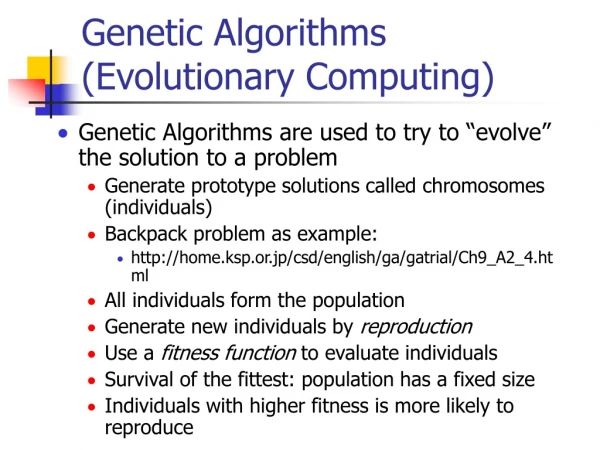
13. Genetic Algorithms: A Tutorial “Genetic Algorithms are good at taking large, potentially huge search spaces and navigating them, looking for optimal combinations of things, solutions you might not otherwise find in a lifetime.” - Salvatore Mangano Computer Design, May 1995

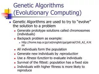
14. Introduction to GA • Evolution in a changing world! • Defining GA! (Goldberg, 1989) Search algorithms based on the principle of natural selection and natural genetics • Survival of the fittest • A natural Perspective • Biological Metaphorsis of GAs

15. In Nature… The strongest survives…

16. GA -Evaluation of solutions We shall look for several alternatives simultaneously. Good location I’ll stick around here I’m redundant here The searchers exchange information during the search, this Information is the basis for the decision regarding their next location

17. Directed search algorithms based on the mechanics of biological evolution • To understand the adaptive processes of natural systems • To design artificial systems software that retains the robustness of natural systems • Provide efficient, effective techniques for optimization and machine learning applications • Widely-used today in business, scientific and engineering circles

18. Components of a GA Aproblem to solve, and ... • Encoding technique (gene, chromosome) • Initialization procedure (creation) • Evaluation function (environment) • Selection of parents (reproduction) • Genetic operators (mutation, recombination) • Parameter settings (practice and art)

19. Simple Genetic Algorithm { initialize population; evaluate population; while Termination Criteria Not Satisfied { select parents for reproduction; perform recombination and mutation; evaluate population; } }

20. Flow chart for Genetic Algorithm Start Generate randomly the popsize times of initial solution Get the input data for No of iterations, cross over probability, mutation probability Solution from Initialization process B Evaluation process – calculate the objective function and find out the fitness value and Selection process Select the chromosome by roulette wheel selection approach Apply Arithmetic cross over Apply mutation Find out the off spring B Is no of iterations are over Take this off spring as initial chromosome stop Y N

21. Outline of the Basic GA • [Start]Generate random population of n chromosomes (suitable solutions for the problem) • [Fitness]Evaluate the fitness f(x) of each chromosome x in the population • [New population] Create a new population by repeating following steps until the new population is complete • [Selection]Select two parent chromosomes from a population according to their fitness (the better fitness, the bigger chance to be selected) • [Crossover] With a crossover probability cross over the parents to form a new offspring (children). If no crossover was performed, offspring is an exact copy of parents. • [Mutation]With a mutation probability mutate new offspring at each locus (position in chromosome). • [Accepting] Place new offspring in a new population • [Replace]Use new generated population for a further run of algorithm • [Test] If the end condition is satisfied, stop, and return the best solution in current population

22. Vertical lines represent solutions (points in search space). The red line is the best solution, Yellow lines are the other ones.

23. Example Problem • Unconstrained Optimization problem max f(x1,x2) = 45.5 + X1 sin (4X1) + X2sin(20X2) -3.0 <=X1<= 12.1 4.1 <=X2<=5.8

25. Representation Encode decision variables into binary strings Length of the strings depends on required precision Domain of Variable Xj is [aj,bj] Required precision is five places after the decimal point. Range of domain should be divided into atleast (bj-aj)*105 size ranges

26. The required bits denoted with mj for a variable is calculated : 2mj-1< (bj-aj)*105<2mj-1 - 1 • Mapping from a binary string to real number for variable xj is: Xj = aj + decimal (substringj)* bj-aj 2mj-1

27. The required bits for variables X1 and X2 are: ((12.1) – (-3.0)) * 10000) = 151000 217 < 151000 <= 218 so, m1 = 18 ((5.8) – (4.1)) * 10000) = 170000 214 < 100000 <= 215 so, m2 = 15 So, m = m1 + m2 = 18 + 15 = 33

28. The total length of chromosome is 33 bits and it is represented as follows: | 33 bits | Vj000001010100101001 101111011111110 | 18 bits | | 15 bits |

29. The corresponding values for X1 and X2 : Binary Number Decimal No. X1 000001010100101001 5417 X2 101111011111110 24318 X1 = -3.0 + 5417 * ((12.1 – (-3.0)) / 218 -1 ) = -2.687969 X2 = 4.1 + 24318 * ((5.8 – (4.1) / 215 -1 ) = -2.687969

30. Back Initial Population – Randomly Generated V1= [000001010100101001 101111011111110] V2= [001110101110011000 000001010100100] V3= [111000111000111000 001111011100011] V4= [111111010100101001 100000011111111] V5= [111101010100101001 101111010000111] V6= [001101010111101001 101111011111110] V7= [111001010100101001 101001011111110] V8= [111111111111101001 100000011111110] V9= [111001010100101001 101111010001111] V10= [000011111100101001 101100000011110]

31. The corresponding decimal values are V1= [X1,X2] = [-2.687969, 5.361653] V2= [X1,X2] = [0.474116, 4.155566] V3= [X1,X2] = [10.419662, 4.772626] V4= [X1,X2] = [6.212122, 4.123212] V5= [X1,X2] = [-2.345678, 4.361773] V6= [X1,X2] = [11.687969, 4.111113] V7= [X1,X2] = [9.682229, 5.533333] V8= [X1,X2] = [-0.123469, 4.891653] V9= [X1,X2] = [11.118889, 4.812453] V10= [X1,X2] = [11.447969, 4.171653]

32. Evaluation • Step 1. Convert the chromosomes’s genotype to its phenotype. • Binary strings into relative real values • Xk= (Xk1, Xk2) , k = 1,2,….,pop_size. • Step 2. Evaluate the Objective fn. f(Xk) • Step 3.Convert the value of Obj. fn. Into fitness. • For Maximization problem, the fitness equal to objective function • eval(Vk) = f(Xk), k = 1,2,….., pop_size

33. The fitness function values of above chromosomes are eval (V1)= f (-2.687969, 5.361653) = 19.233331 eval ( V2 )= f (0.474116, 4.155566) = 17.237891 eval ( V3)= f (10.419662, 4.772626) = 9.781262 - W eval ( V4)= f (6.212122, 4.123212) = 29.881177 - S eval ( V5 )= f (-2.345678, 4.361773) = 15.615118 eval ( V6 )= f (11.687969, 4.111113) = 11.900118 eval ( V7 )= f (9.682229, 5.533333) = 17.012030 eval ( V8 )= f (0.123469, 4.891653) = 19.912734 eval ( V9 )= f (11.118889, 4.812453) = 26.197641 eval ( V10)= f (11.447969, 4.171653) = 10.276541

34. Selection • Roulette wheel approach • Select a new population w.r.to prob. Distr. based on fitness values 1.Calculate fitness value eval (Vk) for each chromosome Vk eval ( Vk ) = f(X), k = 1,2,….pop_size 2.Calculate the total fitness for population pop_size F = ∑ eval ( Vk ) k = j

35. 3.Calculate selection probability Pk for each chromosomeVk : eval ( Vk ) Pk = k = 1, 2, ….., pop_size F 4.Calculate cumulative probability qk for each chromosome Vk : k qk = ∑ Pj, k = 1, 2, ….., pop_size j = 1 The selection process begins by spinning the roulette wheel pop_size times.

36. Selection • Generate a random number r from the range [0,1] • If r <= q1, then select the first chromosome V1; otherwise select the k th chromosome Vk (2<=k<=pop_size) such that qk-1< r < qk The total fitness F of the population is 10 F = ∑ eval ( Vk ) = 178.135372 k = 1

37. Back The probability of a selection pk for each chromosome Vk (k=1,…..,10) is as follows: P1 = 0.111180 P2 = 0.097515 P3 = 0.053839 P4 = 0.165077 P5 = 0.088057 P6 = 0.066806 P7 = 0.100815 P8= 0.110945 P9 = 0.148211 P10= 0.057554 The cumulative probabilities qk for each chromosome Vk (k=1,…..,10) is as follows: q1 = 0.111180 q2 = 0.208695q3 = 0.262534 q4 = 0.427611 q5 = 0.515668 q6 = 0.582475 q7 = 0.683290 q8= 0.794234 q9 = 0.942446 q10= 1.00000 Chromosomes Back Chromosomes

38. Spin the roulette wheel 10 times and each time select a single chromosome for a new population. Let us assume that a random sequence of 10 numbers from the range [0,1] is as follows 0.301431 0.322062 0.766503 0.881893 0.350871 0.583392 0.177618 0.343242 0.032685 0.197577 The first number r1 = 0.301431 is greater than q3 and smaller than q4 meaning that the chromosome V4 is selected for the new population

39. Back The new population after selection process V’1= [111111010100101001100000011111111] (V4) V’2= [111111010100101001100000011111111] (V4) V’3= [111111111111101001100000011111110] (V8) V’4= [111001010100101001101111010001111] (V9) V’5= [111111010100101001 100000011111111] (V4) V’6= [111001010100101001101001011111110] (V7) V’7= [001110101110011000 000001010100100] (V2) V’8= [111111010100101001 100000011111111] (V4) V’9= [000001010100101001 101111011111110] (V1) V’10= [000001010100101001 101111011111110] (V1)

40. Crossover One cut point crossover Probability of Crossover Pc = 0.25 Generate Random Numbers: 0.651234 0.266666 0.288888 0.299999 0.166666 0.566666 0.088888 0.399999 0.701111 0.544444 Choose random numbers less than Pc=0.25 The chromosomes V’5 and V’7were selected for crossover. Generate random number between [0,32] for choosing the position in chromosome

41. Chromosomes selected for crossover V’5=[11111101010010100 1100000011111111] (V4) V’7= [00111010111001100 0000001010100100] (V2) The random position from [0,32] is 17. So, cut from the 17 th gene Chromosomes after crossover V’5= [11111101010010100 0000001010100100] (V4) V’7= [00111010111001100 1100000011111111] (V2)

42. The new population after crossover process • V’’1= [11111101010010100 0000001010100100] (V’5) • V’’2= [00111010111001100 1100000011111111] (V’7) • V’’3= [111111111111101001100000011111110] (V’8) • V’’4= [111001010100101001101111010001111] (V’9) • V’’5= [111111010100101001 100000011111111] (V’4) • V’’6= [111001010100101001101001011111110] (V’7) • V’’7= [001110101110011000 000001010100100] (V’2) • V’’8= [111111010100101001 100000011111111] (V’4) • V’’9= [000001010100101001 101111011111110] (V’1) • V’’10= [000001010100101001 101111011111110] (V’2)

43. Mutation • Flip bit mutation • m=33, pop_size=10 • Probability of mutation Pm=0.01 • Generate sequence of random numbers rk (k= 1,….330) from the range [0 1]

44. The Random position is 105, 4th chromosome, Bit number = 6 Before Mutation V’’4= [111001010100101001101111010001111] (V’9) After Mutation V’’’4= [111000010100101001101111010001111] (V’9)

45. The new population after Mutation process • V’’’1= [11111101010010100 1000001010100100] (V’1) • V’’’2= [00111010111001100 0100000011111111] (V2) • V’’’3= [111111111111101001100000011111110] (V3) • V’’’4= [111000010100101001101111010001111] (V4) • V’’’5= [111111010100101001100000011111101] (V’5) • V’’’6= [111001010100101001101001011111110] (V6) • V’’’7= [101110101110011000100001010100100] (V’7) • V’’’8= [111111010100101001100000011111111] (V8) • V’’’9= [000001010100101001101111011111110] (V9) • V’’’10= [000001010100101000001111011111100] (V’10)

46. The corresponding decimal values (X1,X2) and fitness f(6.167919, 4.107171) = 29.173737 f(6.424242, 4.104451) = 29.771923 f(-3.134919, 4.607171) = 19.171234 f(11.617919, 4.807166) = 5.473734 f(8.167779, 4.176171) = 19.234737 f(9.222219, 5.101271) = 17.155537 f(6.654419, 4.189971) = 29.666737 f(6.88919, 4.234171) = 29.173777 f(-2.117919, 5.87651) = 19.888837 f(0.163229, 4.12371) = 17.188837

47. Termination • Run the test for 1000 generations • Best chromosome in 419th generation V*=(11111000000001110001111010001010110) Eval(V*)= f(11.631407, 5.724824) = 38.818208 X1*=11.631407 X2*= 5.724824 f(X1*,X2*) = 38.818208