Gerschgorin Circle Theorem
Gerschgorin Circle Theorem. Eigenvalues

Gerschgorin Circle Theorem
E N D
Presentation Transcript
Eigenvalues In linear algebra Eigenvalues are defined for a square matrix M. An Eigenvalue for the matrix M is a scalar such that there is a non-zero vector x such that Mx=x. In linear algebra we saw that the Eigenvalues are also roots of the characteristic polynomial det(M-I). For several algorithms in numerical analysis we often need to be able to find a value that is “close” to the value we wish to estimate. This is true for finding solutions of equations as well as Eigenvalues. The Gerschgorin Circle Theorem allows us to estimate how big the Eigenvalues for a matrix can be. Gerschgorin Circle Theorem All the Eigenvalues for a nn matrix M=(mij) are in the union of the disks whose boundaries are circles C1,C2,…,Cn with centers at the points m11,m22,m33,…mnn and the radii are:
The Gerschgorin Circle Theorem basically says that the Eigenvalues for a matrix can not get too far from its diagonal entries. In fact if you remember from linear algebra if the matrix is upper or lower triangular the Eigenvalues are exactly the diagonal entries. Consider the following example. The circles that bound the Eigenvalues are: C1: Center point (4,0) with radius r1 = |2|+|3|=5 C2: Center point (-5,0) with radius r2=|-2|+|8|=10 C3: Center Point (3,0) with radius r3=|1|+|0|=1 The red dots to the right mark the actual location of the Eigenvalues Union of the Circles
In the Gerschgorin Circle Theorem the y-axis is interpreted as the imaginary axis. Since the roots of the characteristic polynomial could be complex numbers they take on the form x+iy where i is the square root of -1. The circles that bound the Eigenvalues are: C1: Center point (1,0) with radius r1 = |0|+|7|=7 C2: Center point (-5,0) with radius r2=|2|+|0|=2 C3: Center Point (-3,0) with radius r3=|4|+|4|=8 We see all the Eigenvalues lie inside the union of all the circles.