Fourier Series and Characteristic functions

1. Fourier Series and Characteristic functions

2. Fourier proposed in 1807 A periodic waveform f(t) could be broken down into an infinite series of simple sinusoids which, when added together, would construct the exact formof the original waveform. Consider the periodic function T = Period, the smallest value of T that satisfies the above equation.

3. To be described by the Fourier Series the waveform f(t) must satisfy the following mathematical properties: • 1. f(t) is a single-value function except at possibly a finite number of points. • 2. The integral for any t0. • 3. f(t) has a finite number of discontinuities within the period T. • 4. f(t) has a finite number of maxima and minima within the period T.

4. Synthesis f(t) t T 2T 3T T is a period of all the above signals Odd Part Even Part DC Part Let ω0=2π/T.

5. Definition A Fourier Seriesis an accurate representation of a periodic signal (when N ∞) and consists of the sum of sinusoids at the fundamental and harmonic frequencies. The waveform f(t) depends on theamplitudeand phaseof every harmonic components, and we can generate any non-sinusoidal waveform by an appropriate combination of sinusoidal functions.

6. Orthogonal Functions Call a set of functions {ϕk}orthogonal on an interval a < t < b if it satisfies Example m =1 0 n = 2 π -π

7. Orthogonal set of Sinusoidal Functions Define ω0=2π/T. We now prove this one

8. Proof m ≠n 0 0

9. Proof m = n 0

10. Define ω0=2π/T. Orthogonal set of Sinusoidal Functions an orthonormal set.

11. Decomposition

12. f(t) 1 -6π -5π -4π -3π -2π -π π 2π 3π 4π 5π Example (Square Wave)

13. f(t) 1 -6π -5π -4π -3π -2π -π π 2π 3π 4π 5π Example (Square Wave)

14. f(t) 1 -6π -5π -4π -3π -2π -π π 2π 3π 4π 5π Example (Square Wave) When series is truncated

15. Harmonics T is a period of all the above signals Even Part Odd Part DC Part

16. Define , called the fundamental angular frequency. Define , called the n-th harmonicof the periodic function. Harmonics

17. Harmonics

18. harmonic amplitude phase angle Amplitudes and Phase Angles

19. Complex Form of the Fourier Series

20. Complex Exponentials

21. Complex Form of the Fourier Series

22. Complex Form of the Fourier Series

23. Complex Form of the Fourier Series

24. Complex Form of the Fourier Series If f(t) is real,

25. amplitude spectrum |cn| n ϕn phase spectrum n Complex Frequency Spectra

26. f(t) A t Example

27. A/5 0 -120π -80π -40π 40π 80π 120π -15ω0 -10ω0 -5ω0 5ω0 10ω0 15ω0 Example

28. A/10 0 -120π -80π -40π 40π 80π 120π -30ω0 -20ω0 -10ω0 10ω0 20ω0 30ω0 Example

29. f(t) A t 0 Example

30. 0 Discrete-time Fourier transform f(t) continuous • Until this moment we were talking continuous periodic functions. • However, probability mass function is a discrete aperiodic function. • One method to find the bridge is to start with a spectral representation for periodic discrete function and let the period become infinitely long. t T 2T 3T discrete

31. Discrete-time Fourier transform • We will take a shorter but less direct approach. Recall Fourier series A spectral representation for the continuous periodic function f(t) Consider now, a spectral representation for the sequence cn, -∞ < n < ∞ • We are effectively interchanging the time and frequency domains. • We want to express an arbitrary function f(t) in terms of complex exponents.

32. Discrete-time Fourier transform • To obtain this, we make the following substitutions in This is the inverse transform continuous discrete

33. Discrete-time Fourier transform To obtain the forward transform, we make the same substitution in

34. Discrete-time Fourier transform • Putting everything together • Sufficient conditions of existence

35. Properties of the Discrete-time Fourier Transform Homework: Prove it Initial value

36. Characteristic functions • Determining the moments E[Xn] of a RV can be difficult. • An alternative method that can be easier is based on characteristic function ϕX(ω). • The function g(X) = exp(jωX) is complex but by defining E[g(X)] = E[cos(ωX) + jsin(ωX)] = E[cos(ωX)] + jE[jsin(ωX)], we can apply formula for transform RV and obtain for those integers not included in SX.

37. Characteristic functions • The definition is slightly different than the usual Fourier transform, called the discrete time Fourier transform, which uses the function exp(-jωk) in its definition. • As a Fourier transform it has all the usual properties. • The Fourier transform of a sequence is periodic with period of 2π.

38. Characteristic functions • CF for finding moments. • Note that we can differentiate the sum “term by term” • Carrying out the differentiation • So that • In fact, repeated differentiation produces the formula for the nth moment as

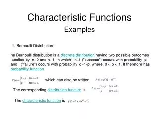
39. Moments of geometric RV: example • Since the PMF for a geometric RV is given by pX[k] = (1 - p)k-1pfor k = 1,2,…, we have that but since |(1-p) exp(jω)| < 1, we can use the result For z a complex number with |z| < 1 to yield the CF Note that CF is periodic with period 2π.

40. Moments of geometric RV: example • Let’s find the mean(first moment) using CF. • Let’s find the second moment using CF and then variance. Where D = exp(-jω) - (1-p). Since D|ω=0 = p,we have that

41. Expected value of binomial PMF • By finding second moment we can find variance a b binomial theorem

42. Properties of characteristic functions • Property 1. CF always exists since • Proof • Property 2. CF is periodic with period 2π. • Proof: For m an integer since exp(j2πmk) = 1 for mk an integer.

43. Properties of characteristic functions • Property3. The PMF may be recovered from the CF. • Given the CF, we may determine the PMF using • Proof: Since the CF is the Fourier transform of a sequence (although its definition uses a +j instead of the usual -j), it has an inverse Fourier transform. Although any interval of length 2π may be used to perform the integration in the inverse Fourier transform, it is customary to use [-π, π].

44. Properties of characteristic functions • Property 4. Convergence of characteristic functions guarantees convergence of PMFs (Continuity theorem of probability). • If we have a sequence of CFs φnX(ω) converge to a given CF, say φX(ω), then the corresponding sequence of PMF, say pnX[k], must converge to a given PMF say pX[k]. • The theorem allows us to approximate PMFs by simpler ones if we can show that the CFs are approximately equal.

45. Application example of property 4 • Recall the approximation of the binomial PMF by Poisson PMF under the conditions that p 0 and M  ∞ with Mp = λ fixed. • To show this using the CF approach we let Xb denote a binomial RV. And replacing p by λ/M we have as M ∞.

46. Application example of property 4 • For Poisson RV XP we have that • Since φXb(ω)  φXp(ω) as M ∞, by property 4 we must have that pXb[k]  pXp[k] for all k. Thus, under the stated conditions the binomial PMF becomes the Possion PMF as M  ∞.

47. Practice problems 1. Prove that the transformed RV has an expected value of 0 and a variance of 1. 2. If Y = ax + b, what is the variance of Y in terms of the variance of X? 3. Find the characteristic function for the PMF pX[k] = 1/5, for k = -2,-1,0,1,2. 4. A central moment of a discrete RV is defined as E[(X – E[X])2] , for n positive integer. Derive a formula that relates the central moment to the usual (raw) moments. 5. Determine the variance of a binomial RV by using the properties of the CF. Assume knowledge of CF for binomial RV.

48. Homework 1. Apply Fourier series to the following functions on (0; 2π) a. b. c. 2. Find the second moment for a Poisson random variable by using the characteristic function exp⁡[λ(exp(jω)-1)]. 3. A symmetric PMF satisfies the relationship pX[­-k] = pX[k] for k = …,-1,0,1,…. Prove that all the odd order moments, E[Xn] for n odd, are zero.