Download
1 / 103
1.05k likes | 1.25k Views
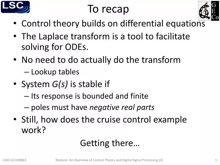
To recap. Control theory builds on differential equations The Laplace transform is a tool to facilitate solving for ODEs . No need to do actually do the transform Lookup tables System G(s) is stable if Its response is bounded and finite poles must have negative real parts

E N D
To recap • Control theory builds on differential equations • The Laplace transform is a tool to facilitate solving for ODEs. • No need to do actually do the transform • Lookup tables • System G(s) is stable if • Its response is bounded and finite • poles must have negative real parts • Still, how does the cruise control example work? Getting there… Matone: An Overview of Control Theory and Digital Signal Processing (2)
Recall What is the transfer function of a system whose input and output are related by the following differential equation? Matone: An Overview of Control Theory and Digital Signal Processing (2)
Recall Given the system’s transfer function determine the system’s differential equation to input . Matone: An Overview of Control Theory and Digital Signal Processing (2)
Recall Determine which of the following transfer functions represent stable systems and which represent unstable systems. Use MATLAB’s step to verify your answer. Matone: An Overview of Control Theory and Digital Signal Processing (2)
Another example y B M k x A simple mechanical accelerometer is shown below. The position y is with respect of the case, the case’s position is x. What is the transfer function between the input acceleration and the output Y? Matone: An Overview of Control Theory and Digital Signal Processing (2)
Control Theory 2 The response of a stable system G(s) is characterized by its Amplitude and Phase shift to a sinusoidal excitation Matone: An Overview of Control Theory and Digital Signal Processing (2)
Frequency response This is how we measure transfer functions X It can be shown that if then where is the amplitude response and is the phase shift Matone: An Overview of Control Theory and Digital Signal Processing (2)
Frequency response The dynamic behavior of a physical system can be determined by measuring its transfer function with a sinusoidal excitation Magnitude and phase response are a function of frequency ( Frequency-response helps to understand the stability criteria Matone: An Overview of Control Theory and Digital Signal Processing (2)
Graphical analysis tool: Bode Plot • Common graphical representation of transfer function • is complex • plot of magnitude and phase • Convention • Log-log scale for magnitude vs. frequency (Hz) • Semi-log scale for phase (deg) vs. frequency (Hz) • Other conventions • Magnitude in dB () vs. angular frequency (rad/s) Matone: An Overview of Control Theory and Digital Signal Processing (2)
Bode plot: Matone: An Overview of Control Theory and Digital Signal Processing (2)
bodeexamples.m Matone: An Overview of Control Theory and Digital Signal Processing (2)
Bode plot: Matone: An Overview of Control Theory and Digital Signal Processing (2)
bodeexamples.m Matone: An Overview of Control Theory and Digital Signal Processing (2)
Bode plot: Matone: An Overview of Control Theory and Digital Signal Processing (2)
bodeexamples.m Matone: An Overview of Control Theory and Digital Signal Processing (2)
Bode plot: Matone: An Overview of Control Theory and Digital Signal Processing (2)
bodeexamples.m Matone: An Overview of Control Theory and Digital Signal Processing (2)
Bode plot: Matone: An Overview of Control Theory and Digital Signal Processing (2)
bodeexamples.m Matone: An Overview of Control Theory and Digital Signal Processing (2)
bodeexamples.m Matone: An Overview of Control Theory and Digital Signal Processing (2)
bodeexamples.m Matone: An Overview of Control Theory and Digital Signal Processing (2)
Bode plot: SHO Matone: An Overview of Control Theory and Digital Signal Processing (2)
bodeexamples.m Matone: An Overview of Control Theory and Digital Signal Processing (2)
bodeexamples.m Matone: An Overview of Control Theory and Digital Signal Processing (2)
bodeexamples.m Matone: An Overview of Control Theory and Digital Signal Processing (2)
Bode plots for more complicated TFs? Break it into simpler parts In general a transfer function can be re-written in terms of simpler ones (of 2nd order at most) then Matone: An Overview of Control Theory and Digital Signal Processing (2)
Example Let’s draw the bode plot for where Matone: An Overview of Control Theory and Digital Signal Processing (2)
Example Matone: An Overview of Control Theory and Digital Signal Processing (2)
Log(f) 10Hz 0.1Hz 1Hz Log(f) Matone: An Overview of Control Theory and Digital Signal Processing (2)
Log(f) 10Hz 0.1Hz 1Hz Log(f) Matone: An Overview of Control Theory and Digital Signal Processing (2)
bodeexamples.m Matone: An Overview of Control Theory and Digital Signal Processing (2)
>> z=-2*pi*0.1; • >> p=-2*pi*[1 10]; • >> k=500; • >> G=zpk(z,p,k); • >> [m,p]=bode(G, w); bodeexamples.m Matone: An Overview of Control Theory and Digital Signal Processing (2)
Exercise Sketch bode plot for the following TF What is the DC gain (gain for )? What is the gain for ? Confirm results with MATLAB Matone: An Overview of Control Theory and Digital Signal Processing (2)
Exercise Sketch bode plot for the following TF What is the DC gain (gain for )? What is the gain for ? Confirm results with MATLAB Matone: An Overview of Control Theory and Digital Signal Processing (2)
Exercise Sketch bode plot for the following TF What is the DC gain (gain for )? What is the gain for ? Confirm results with MATLAB Matone: An Overview of Control Theory and Digital Signal Processing (2)
So far… • A system’s TF is a complex function • Can be represented in terms of its magnitude and phase • Bode plots • Help visualize the TF • Plot of magnitude vs. frequency and phase vs. frequency. • Different conventions • We have explored Bode plots of basic TFs • Bode plot of more complex TFs can be expressed in terms of simpler terms Matone: An Overview of Control Theory and Digital Signal Processing (2)
General Stability Criterion The feedback control system is stable if and only if all the poles of the closed loop transfer function have a negative real part. Otherwise the system is unstable. Matone: An Overview of Control Theory and Digital Signal Processing (2)
In general r e + G(s) - c H(s) Closed loop gain Open loop gain • Stability: the poles’ real part of must be negative Matone: An Overview of Control Theory and Digital Signal Processing (2)
Loop stability and design r e + G(s) - c H(s) • If the system is unstable, • We can’t change but • We can design a different controller so as to make the system stable • But how should we change H? Let’s look closely at the root of the problem Matone: An Overview of Control Theory and Digital Signal Processing (2)
The problem r e + G(s) - c H(s) If ever becomes then system is unstable Matone: An Overview of Control Theory and Digital Signal Processing (2)
The general shape of r e + G(s) has a limited bandwidth. - c Outside bandwidth: Within bandwidth: H(s) Matone: An Overview of Control Theory and Digital Signal Processing (2)
The general shape of “Bandwidth” DC gain Unity gain Unity Gain Frequency (UGF): Log(f) Log(f) Matone: An Overview of Control Theory and Digital Signal Processing (2)
Stability Criteria A closed loop system is stable if the unity gain frequency is lower than the crossing. Log(f) UGF Stable crossing Log(f) Matone: An Overview of Control Theory and Digital Signal Processing (2)
Stability Criteria:Rule of Thumb The system is (almost always) stable if at the unity gain frequency. Log(f) Slope at UGF: Stable Log(f) Matone: An Overview of Control Theory and Digital Signal Processing (2)
Nyquist stability criterion The closed loop system is stable if the polar plot of the open loop transfer function does not encircle the point. nyquist_example1.m • >> G=10*tf(10,[1 10]; • >> nyquist(G) Matone: An Overview of Control Theory and Digital Signal Processing (2)
Nyquist stability criterion The closed loop system is stable if the polar plot of the open loop transfer function does not encircle the point. • Checking the step response of 1/(1+Gol) nyquist_example1.m Matone: An Overview of Control Theory and Digital Signal Processing (2)
Back to cruise control Let’s inspect the system’s loop stability. Recall • Mass m = 1000 kg • Coefficient for air friction b = 50 kg/s θ vr e + f H - K - + v G c Matone: An Overview of Control Theory and Digital Signal Processing (2)
Cruise control: Bode plot of cruise_freqdomain.m UGF @160 mHz Matone: An Overview of Control Theory and Digital Signal Processing (2)
Cruise control: Nyquist plot of cruise_freqdomain.m Matone: An Overview of Control Theory and Digital Signal Processing (2)
With a little algebra: Matone: An Overview of Control Theory and Digital Signal Processing (2)