Download
1 / 1
10 likes | 132 Views
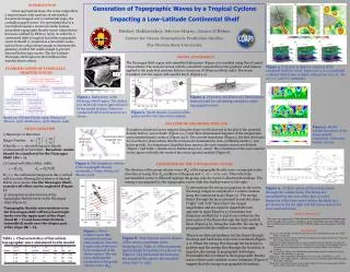
1. 3. Figure 3. Geometry and fluxes of a fixed volume element used for calculating energetics of the topographic waves. Figure 2. Model domain. Location of the points used for the time series analysis. SCALE ANALYSIS 1) Barotropic vs Baroclinic Burger Number:

E N D
1 3 Figure 3. Geometry and fluxes of a fixed volume element used for calculating energetics of the topographic waves. Figure 2. Model domain. Location of the points used for the time series analysis. SCALE ANALYSIS 1) Barotropic vs Baroclinic Burger Number: When Bu >> 1, the shelf response should predominantly be baroclinic. Baroclinic modes should be considered for the Nicaragua Shelf (Bu > 1). 2) Coastal wall effect (Allen, 1980): If > 1, the continental margin acts like a vertical wall to a wave allowing the existence of internal Kelvin wave modes. For the Nicaragua Shelf, coastal wall effect can be neglected (Figure 1). Bottom intensified (trapped) wave Ri > L Barotropic shelf wave, Ri < L ENERGETICS OF THE TOPOGRAPHIC WAVES The direction of the group velocity vector (Cg) of the topographic Rossby wave corresponds to the direction of energy flux. Cg and K are orthogonal and Thus when the wavenumber vector is directed upslope the group velocity vector is directed downslope. The energy is propagated by the topographic waves with the shallow water to the right. K 3) Anticipated modal structure of the topographic Rossby waves on the Nicaragua slope (Figure 6): Topographic Rossby wave motions over the Nicaragua shelf will have barotropic mode over the upper part of the slope (local Ri < L) and baroclinic (bottom-intensified) mode over the deeper part of the slope (Ri > L). Table 1. Characteristics of baroclinic topographic wave simulated in the model Cg Generation of Topographic Waves by a Tropical Cyclone Impacting a Low-Latitude Continental Shelf INTRODUCTION Given appropriate slope, the ocean responds to a tropical storm with motions of sub-inertial frequencies trapped over a continental slope, the coastally trapped waves. It is speculated that in a low-latitude region a storm can excite bottom-intensified topographic Rossby waves whose theory has been outlined by Rhines (1970). In order for a continental shelf to support baroclinic topographic waves it should (1) respond as a baroclinic ocean, and (2) have a slope steep enough to dominate the planetary -effect but small enough to prevent internal Kelvin-type modes. The low-latitude Nicaragua shelf region in the Caribbean Sea matches those criteria. Dmitry Dukhovskoy, Steven Morey, James O’Brien Center for Ocean-Atmospheric Prediction Studies The Florida State University MODEL EXPERIMENT The Nicaragua Shelf region with simplified bathymetry (Figure 2) is modeled using Navy Coastal Ocean Model. The model is forced with the wind field computed from the gradient wind balance applied to the analytical pressure field in a hurricane (O’Brien and Reid, 1967). The storm translates over the region with speed 6 km/h (Figure 4 a). Figure 4. Evolution in time (in columns) of the simulated fields (in rows). Upper row (a, b, c): potential -density field at 300 m depth. Bottom row (d, e, f): the 22°, 11°, and 6°C isotherms. CLASSIFICATION OF COASTALLY TRAPPED WAVES Figure 1. Bathymetry of the Nicaragua Shelf region. The dashed box marks the region approximated by the model domain. Values for coastal wall effect scale analysis are shown. Based on: Gill and Clarke, 1974; Wang and Mooers, 1976; Huthnance, 1978; Mysak, 1980. ANALYSIS OF THE MODEL RESULTS Formation of internal waves trapped along the slope is well observed in the plot of the potential density field at -300 m depth (Figure 4 a-c) and three-dimensional diagrams of the temperature and potential density surfaces (Figure 4 d-f). The wavelet transforms (Figure 5, the first 180 hours are not shown) demonstrate that the motions are dominated by slow-oscillating modes (> 100 hours period). For frequencies identified from spectra, the wave-number vectors are derived (Figure 7 and Table 1, details are in Dukhovskoy et al., 2007). The orientation of the wave-number vector agrees well with the result of the rotary spectral analysis (Figure 8). Figure 5. Morlet wavelet transform of the along-isobath component of the near-bottom velocity. Figure 6. The alongshore velocity of the topographic Rossby wavemode 1. From: Wang and Mooers, 1976. To demonstrate the energy propagation by the waves, the energy budget is computed for a volume element along the continental slope (Figure 3). The energy fluxes through the faces oriented across the slope (“right” and “left” faces) have the largest magnitudes and are equal in magnitude and opposite in sign (Figure 9 a). Dominant low-frequency oscillations (~150 h) are evident in the time series of the fluxes through the right and left faces (Figure 9 b). Along the isobaths, the energy is propagated with the shallow water to the right. Figure 9. (a) Time series of the energy fluxes through the volume faces. The fluxes are normalized by the area of the face (J/s m2). Segments of the time series within the black box are shown in (b) for right and left faces, and (c) for front and back faces. ACKNOWLEDGMENTS This study was supported by NASA Physical Oceanography and by funding through the NOAA ARC. The authors would like to thank Paul Martin and Alan Wallcraft at the Naval Research Laboratory for the NCOM development and assistance with the model. Figure 7. Wave-number vector (K) estimates from time series analysis. Note the length scale of the wave is the reciprocal of the shown vectors. The red arrow indicates the orientation of the group velocity vector (Cg). REFERENCES Allen, J.S., 1980. Models of wind-drive currents on the continental shelf. Ann. Rev. Fluid Mech., 12, 389-433. Buchwald, V.T., and J.K. Adams, 1968. The propagation of continental shelf wavs. Proc. Roy. Soc. London, A305, 235-250. Charney, J.G., 1955. The generation of ocean currents by wind. J. Mar. Res., 14, 433-498. Dukhovskoy, D.S., S.L. Morey, and J.J. O’Brien, 2007. Generation of Topographic Waves by a Tropical Cyclone Impacting a Low-Latitude Continental Shelf. Cont. Shelf Res., accepted. Gill, A.E., and A.J. Clarke, 1974. Wind-induced upwelling, coastal currents and sea level changes. Deep-Sea Res. 21, 325-345. Mysak, L.A., 1980. Topographically trapped waves. Ann. Rev. Fluid Mech. 12, 45-76. Rhines, P.B., 1970. Edge-, bottom-, and Rossby waves in a rotating stratified fluid, Geophys. Fluid. Dyn. 1, 273-302. Wang, D.-P., and C.N.K. Mooers, 1976. Coastal-trapped waves in a continuously stratified ocean, J. Phys. Oceanogr. 6 (6), 853-863. There is an obvious tendency for the fluxes through the front and back faces to be anti-correlated (Figure 9 c). When the energy flux through the back face is positive and the energy flux through the front face is negative, the energy is propagated downslope. Presumably this is related to the topographic Rossby waves whose wave-number vector estimates (Figure 7) suggest that the energy is propagated downslope. Figure 8. Near-bottom current ellipses of the rotary constituent at the frequency (, Table 1) of the maximum spectral peak for points 1 to 4 shown in Figure 2. The horizontal bar indicates the length of the axis for the specified value (cm2/ s2 cph).