Download
1 / 62
620 likes | 750 Views
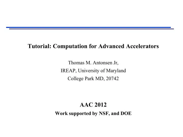
Tutorial: Computation for Advanced Accelerators Thomas M. Antonsen Jr, IREAP, University of Maryland College Park MD, 20742 AAC 2012 Work supported by NSF, and DOE. Computation has become integral to Accelerator Science. Why is Computation Important ?

E N D
Tutorial: Computation for Advanced AcceleratorsThomas M. Antonsen Jr, IREAP, University of MarylandCollege Park MD, 20742AAC 2012Work supported by NSF, and DOE
Computation has become integral to Accelerator Science Why is Computation Important ? - Understanding of basic physical processes - Understanding and diagnosing particular experiments - Designing improved experiments - Optimizing designs
Areas of Progress Improved Physics Models Find better descriptions of what’s going on inside a an accelerator More Efficient Algorithms Solve the governing equations with fewer operations and/or less memory usage. New Computing Architectures Restructure your code to take advantage of new hardware.
Examples of Areas where Computation is Important Particle trajectories in analytic fields* Space charge fields* Magnetic fields due to currents in coils RF fields in cavities and waveguides Radiation generated by energetic particles Multipactor Plasma-Based Acceleration and more *See R. Rynehttp://uspas.fnal.gov/materials/09UNM/ComputationalMethods.pdf
Unstructured mesh Structured mesh Meshes and Grids Calculations are carried out on digital computers Time is discretized Space may also be discretized - meshes or grids If field is a dynamical variable (Maxwell’s Equations) a mesh is needed If field describes pair-wise interaction forces (Coulombs law) it can be calculated with or without a grid.
Tree Code Calculation of Coulomb interaction without gridsJ. Barnes and P. Hut,“A hierarchical force-calculation algorithm,”Nature, vol. 324, pp. 446–449, 1986 Direct application of Coulomb’s law to N particles requires O(N2) operations. Not practical for large N. Tree code: Divide domain into cells Each cell has fewer than NL particles Particles within same cell interact pairwise Particles in different cells interact through multipole moments O(NlogN) operations possible
Mesh Types Structured Mesh Unstructured Mesh Complex geometries may be represented using a multi-block representation: conformal meshes: boundary of mesh conforms with physical boundary
Finite Integration Technique Applicable to orthogonal Cartesian mesh Degrees of freedom are integrals of fields over appropriate mesh elements Suffers due to non-conformal representation of geometry Finite Element Method Applicable to curvilinear mesh(structured or unstructured) Field described by interpolating basis functions in each cell Solves integral (weak) form of 2nd order differential equations Evaluates matrix elements using overlap integrals of basis & test functions Large number of coupling terms Existing Discretization Techniques Basis & test functions 1 0 -½ ½
• Widely used • Simple (explicit) • Second order accurate • Stable if Dt <cdx Fields and Structured Mesh for FDTD solution of Maxwell’s Equations Yee Mesh (1966) Electric fields defined on edges Magnetic fields defined on faces Electric fields defined at integer time steps Magnetic fields defined at half integer time steps
Leap Frog Explicit FDTDSolutions to Maxwell’s Equation time differencing Alternately apply Faraday’s law to faces Explicit: knowing E at time t allows for direct calculation of H at time t+Dt/2
Finite Differencing Plane Waves Assume all fields vary as Dispersion relation for Plane waves Continuous FDTD
Stability - Courant Freidricks Lewy Condition (CFL) Dispersion Relation Left side < Maximum of Right Side Stable if CFL Condition
Dispersion and Accuracy Dispersion in discrete system is periodic. Departures from continuous system are quadratic in Dt, D. Waves have phase velocity <c Numerical Cerenkov Radiation - Requires filter
Conducting Boundaries on Structured Grids When boundary does not coincide with mesh FDTD must be modified. Without modification errors of order D are introduced. Boundary S. Dey, R. Mittra, A locally conformal finite-difference time-domain (FDTD) algorithm modeling modeling three-dimensional perfectly conducting objects, IEEE Microwave Guided Wave Lett. 7 (1997) 273 Problem: If cells are small CFL condition is violated Separate modification to compute surface losses.
ADI (Alternating Dimension Implicit) Solutions to Maxwell’s Equation) Scalar: Douglas, Peaceman, and Ratchford (1955) ME: Namiki T (1999), Zheng, Chen, Zhang (2000) time differencing • Split time steps • Recently developed • Complex (implicit) • Not subject to Courant condition, Dt > cdx Second half of time step has x, y, and z permuted
Leapfrog ADI-FDTD equationsS. Cooke et al (2009) • Electric and magnetic field terms are offset in time • Electric fields only appear on the half time steps • Magnetic fields only appear on the full time steps • Still need to solve six tri-diagonal equations per time step • 3 for the E-components, 3 for the H-components • ADI-FDTD uses 6 for the E-components (3 components, 2 half steps) • No additional explicit equations are necessary Tri-diagonal operators “curl” terms
PIC Algorithm - From Plasma Physics via Computer Simulation C. K. Birdsall and A. B. Langdon FDTD ME in here
Integration of Equations of Motion Basic Leap Frog: p and x known on staggered time grid Modified for Lorenz Force: “Boris Push” Half step with E Full step with B Half step with E
Interpolation of Fields and Accumulation of Currents and Charges E and J are known on the same grid, but are staggered in time Forces interpolated from grid to location of particles Particle contribution to current density accumulated on grid. Algorithm should conserve charge. J.Villasenor and O.Buneman. Computer Physics Communications, 69. 306-316, (1992)
FDTD-PIC Time-stepping loop S. Cooke NRL IVEC 2012 21 Charge is not computed,only current is used. Space charge fields occur only through integration of Maxwell’s equations. Charge-conserving methodsdo this exactly – no need fordivergence-cleaning. H P E X J Advance H Assign external current sources Add new particles Advance P, then X (accumulating J) Remove dead particles Advance E
Plasma Based Accelerators • Direct Acceleration in Modulated Channels
Physical Processes Important • Relativistic Motion • Plasma Wave Generation / Cavitation • Laser Self Focusing / Scattering • Ionization Not Important • Turbulence - most plasma particles interact for a short time, several plasma periods, then leave Our job is “relatively” easy. Simulation has played an important role in the development of the field. Guiding our understanding Designing new experiments
Relevant Time Scales (LWFA) • Laser Period l =800 nm TL = 2.7 fs • Driver Duration ~ Plasma Period TD = 50 fs • Propagation Time (driver evolution, L= 1 cm) TP = 3.3 104 fs (driver evolution, L= 1 m) TP = 3.3 106 fs • Disparity in time scales leads to both complications and simplifications Propagation Time >> Driver Duration >> Laser Period TP >> TD >> TL
MODELS APPROACHES / APPROXIMATIONS • Laser Full EM - Laser Envelope • Plasma Particles - Fluid Full Lorenz force - Ponderomotive Dynamic response - Quasi-static
Hierarchy of Descriptions 1. Full Format Particle in Cell (PIC) - Relativistic equations of motion for macro-particles - Maxwell’s Equations on a grid - Most accurate but most computationally intensive • Laser Full EM - Laser Envelope • Plasma Particles - Fluid Full Lorenz force - Ponderomotive Dynamic response - Quasi-static
t=L/c z=0 z=L Windows and Frames Three versions: - Lab Frame - Moving Window - Boosted Frame Lab Frame - # Grids NLF = (L/dz)2 ~ (L/l)2 dt=dz/c Moving Window - # Grids NMW = (LD/L) NLF grid must resolve l - LD Propagation distance Pulse length
Boost - g t=L/c t' =L/gc z'=0 z' =-gLD dz' = gdz z=0 z=L Boosted FrameJ-L Vay, PRL98, 130405 (2007) Lab Frame dt' = gdt • Qualifications: • -no backscatter. In boosted frame gives upshift. Requires smaller dz' • transverse grid size sets limit on • dt' < dx' /c= dx /c Boosted frame - # grids NBF = g-2 NMW Optimumbased on 1D makes simulation “square”
Using conventional PIC techniques, 2-3 orders of magnitude speedup reported in 2D/3D by various groups Osiris: trapped injection Vorpal: external injection w/ beam loading Warp: external injection wo/ beam loading • Reported speedups limited by various factors: • laser transverse size at injection, • statistics (trapped injection), • short wavelength instability (most severe). J-L Vay
2. Full EM vs. Laser EnvelopeDriver Duration >> Laser Period TD >> TL • Required Approximation for Laser envelope: wlasertpulse >> 1, rspot >> l wp /wlaser <<1 • Advantages of envelope model: -Larger time steps Full EM stability: Dt < Dx/c Envelope accuracy: Dt < 2pDx2/lc - No unphysical Cherenkov radiation - Further approximations • Advantages of full EM: Includes Stimulated Raman back-scattering Also direct acceleration
• Laser + Wake field: E = E + E laser wake • Vector Potential: A = A ( , x , t ) exp i k + c . c . x x laser 0 0 ^ • Laser Frame Coordinate: = ct – z x Necessary for: Raman Forward Self phase modulation vg< c Drop (eliminates Raman back-scatter) Laser Envelope Approximation • Envelope equation:
2 2 2 k c + w Extended Paraxial – p ^ v ( ) = c / 1 + w g 2 2 w 1 / 2 2 2 2 k c + w True : p ^ v ( ) = c 1 – w g 2 w Requires : 2 2 2 2 k c , < < w w p ^ Validity of Envelope Equation Extended Paraxial approximation - Correct treatment of forward and near forward scattered radiation - Does not treat backscattered radiation - If grid is dense enough can treat Dw ~ w
• Full Lorenz: • Separation of time scales d p v B ´ E = E + E i i = q E + laser wake c dt x ( t ) = x ( t ) + x ( t ) • Requires small excursion d x i = v i dt x ( t ) E < < E × Ñ laser laser • Ponderomotive Equations v B d p ´ wake = q E + + F c wake p dt 2 2 q A p laser = 1 + + g 2 2 2 m c m c 2 q A 2 m c laser F = – Ñ p 2 m c 2 g 3. Full Lorenz Force vs. Ponderomotive Description
Deposit Sources j and r Deposit Source nq2/<gm> Advance Fields (Maxwell’s Equations) Advance Laser (Envelope Equation) Lorentz Push Ponderomotive Push + Ponderomotive Guiding Center PIC Code: TurboWAVE D.F. Gordon, et al. , IEEE TRANSACTIONS ON PLASMA SCIENCE , V 28 , 1224-1232 ( 2000 ) Fields are separated into high and low frequency components. The low frequency component is treated as in an ordinary PIC code. The high frequency component is treated using a reduced description which averages over optical cycles. Low Frequency Cycle High Frequency Cycle
INF&RNO(INtegrated Fluid & paRticle simulatioN cOde)C. Benedetti at al. (LBNL) 2D cylindrical + envelope for the laser (ponderomotive approximation) full PIC/fluid description for plasma particle (quasi-static approx. is also available) switching between PIC/fluid modalities (hybrid PIC-fluid sim. are possible) dynamical particle resampling to reduce on-axis noise 2nd order upwind/centered FD schemes + RK2/RK4 (& Implicit) for time integration linear/quadratic shape functions for force interpolation/charge deposition high order low-pass compact filter for current/field smoothing “BELLA”-like runs (10GeV in ~ 1m) become feasible in a few days on small machines FLUID PIC 35
t Electron transit time: pulse = d t ¶ ¶ = + c – v + v × Ñ e 1 – v / c z dt t ^ ^ c ¶ z ¶ x Plasma electron c - vz Trapped electron 4. Quasi - Static vs. Dynamic WakeP. Sprangle, E. Esarey and A. Ting, Phys. Rev. Lett. 64, 2011 (1990) Laser Pulse PlasmaWake Electron transit time << Pulse modification time Advantages: fewer particles, less noise (particles marched in ct-z) Disadvantages: particles are not trapped
x=ct-z r Two Time Scales 1. “fast time” t ~ TD ~ wp-1 particle trajectories and wake fields determined 2. “slow time” laser pulse evolves diffraction self-focusing depletion Quasi Static Simulation Code WAKEP. Mora and T. M. Antonsen Jr. - Phys Plasma 4, 217 (1997) Particle trajectories
QuickPIC: 3D quasi-static particle code • Description • Massivelly Parallel, 3D Quasi-static particle-in-cell code • Ponderomotive guiding center for laser driver • 100-1000+ savings with high fidelity • Field ionization and radiation reaction included • Simplified version used for e-cloud modeling • Developed by UCLA + UMaryland + IST Examples of applications • Simulations for PWFA experiments, E157/162/164/164X/167 (Including Feb. 2007 Nature) • Study of electron cloud effect in LHC. • Plasma afterburner design up to TeV • Efficient simulation of externally injected LWFA • Beam loading studies using laser/beam drivers • New Features • Particle tracking • Pipelining • Parallel scaling to 1,000+ processors • Beta version of enhanced pipelining algorithm: enables scaling to 10,000+ processors and unprecedented simulation resolution down to nm Chengkun Huang: huangck@ee.ucla.edu http://exodus.physics.ucla.edu/ http://cfp.ist.utl.pt/golp/epp
Particles and Wake QUASI-STATIC CODE STRUCTURE Laser “slow time - t” “fast time x=ct-z”
• Hamiltonian: : PARTICLES CONTINUEDconstant of motion • Weak dependence on “t” in the laser frame • Introduce potentials Transverse Dynamics • Algebraic equation:
Intensity LOCAL FREQUENCY MODIFICATIONM. Tsoufras, PhD Thesis, UCLA Frequency shift is proportional to propagation distance ne Assume complete cavitation Relative frequency shift is unity at the dephasing distance
Comparison of Spectra; Modified Paraxial, Full-wave, and FDTD-PIC
Conclusions • Numerical simulation of Laser-Plasma interactions is a powerful tool • A variety of models and algorithms exist first principles reduced modles • Field is still advancing with new developments Boosted Frame Calculations speed-up ~ g2 3D Parallel Quasi-static speed-up ~ [w0/wp]2 GPUs
WAKE - CavitationP. Mora and T. Antonsen PHYSICAL REVIEW E, Volume: 53 R2068 (1996) Intensity Density Trajectories Complete cavitation Suppression of Raman instability Stable propagation for 30 Rayleigh lengths
3 cm ~ 90 corrugations ~ 40 TR Wake simulation of pulse propagation in corrugated plasma channels See WG #1 B. Layer Wed. PM, J. Palastro Thu. AM =800 nm wch=15 m ao=.35 t=1 ps no=7x1018 cm-3 =.9 m=.035 cm 150 m density intensity t=0 TR t=15 TR t=30 TR Upper: corrugated Lower: smooth Suppression of Raman Instability
QUICKPIC Quasi-Static Plasma Particles Wake Fields Dynamic Beam Particles Laser Field
Second Order Accurate Split-Step Scheme Laser Advance Axial (dt) Transverse (dt) Axial (dt) Transverse (dt) Axial (dt/2) push particles push particles Plasma Particle Advance time-s time-t t t t+dt t+dt
Verification : Full PIC vs. Quasi-static PIC Benchmark for different drivers: QuickPIC vs. Full PIC • Excellent agreement with full PIC. • 100 to 10000 times savings in CPU needs • No noise issues and no unphysical Cerenkov radiation e- driver e+ driver e- driver with ionization laser driver 100 to 10000 CPU savings with “no” loss in accuracy