Download
1 / 7
70 likes | 336 Views
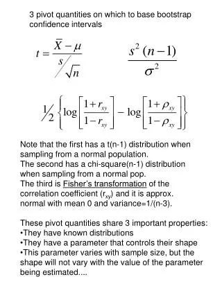
3 pivot quantities on which to base bootstrap confidence intervals. Note that the first has a t(n-1) distribution when sampling from a normal population. The second has a chi-square(n-1) distribution when sampling from a normal pop. The third is Fisher’s transformation of the

E N D
3 pivot quantities on which to base bootstrap confidence intervals • Note that the first has a t(n-1) distribution when • sampling from a normal population. • The second has a chi-square(n-1) distribution • when sampling from a normal pop. • The third is Fisher’s transformation of the • correlation coefficient (rxy) and it is approx. • normal with mean 0 and variance=1/(n-3). • These pivot quantities share 3 important properties: • They have known distributions • They have a parameter that controls their shape • This parameter varies with sample size, but the • shape will not vary with the value of the parameter • being estimated....
As the Student’s t distribution “takes away the mean and divides by the s.e. of the sample mean”, so we codify this process and call it Studentization for any estimator t of q . We’ll use the bootstrap form of the Studentized estimate to construct various bootstrap confidence intervals...
So here’s the way to do this for the mean. • compute the sample mean and sample s.d. from the original data • obtain a bootstrap sample of size n from the original data and compute the bootstrap mean, and the bootstrap standard deviation, sb. • now compute the bootstrap t-pivot quantity: • now repeat this step at least 1000 times to get the bootstrap distribution of tb . • let tb, .025 and tb, .975 be the .025 and .975 quantiles of the bootstrap distribution of tb . Construct the 95% confidence interval for m as • Now implement this in R... try with the “latch failure” data in Table 1.2.1
Bootstrap confidence intervals for the population standard deviation, s, can be done with the c2-pivot: • If the sample is from a normal distribution, then the c2-pivot has a chi-square distribution with n-1 degrees of freedom and a 95% confidence interval for sigma can be computed as: • If normality is not a reasonable assumption, then we’ll use the bootstrap as follows: • compute the sample variance s2 for the original sample data. • bootstrap the sample of size n and compute the bootstrap sample variance and the bootstrap c2-pivot quantity (here, sb2 is the bootstrap sample variance) • now repeat 1000 times or more to get the bootstrap distribution of the bootstrapped c2-pivots
then the bootstrap 95% CI for the population variance is • take the square root if you want confidence intervals for sigma... • Implement this in R... again on the Table 1.2.1 data. Here are the problems from the textbook that are due at the final exam time. Be sure to write up the solution so I can tell that you understand the methods and the context of the problem. Include appropriate R output to illustrate your solutions... p.106: #6 p.141ff: #4,5,6 (second part), 7,9 p.189ff: #1,3,4,5,7,8,9(a),12,13 p.298ff: #1,5,7 On the last class day I will give you some data that will form the basis for the final exam the next week. See page 258 for a chart of Coverage Percentages in a simulation done by the author for various underlying distributions - make sure you understand the conclusions of that discussion…
See section 8.3 for a discussion of three additional methods for computing bootstrap confidence intervals in more generality… The three methods are: • Percentile method • Residual method • BCA method (BCA=bias corrected and accelerated) • Suppose we are trying to estimate the unknown population parameter - use based on a sample of size n from the population. • The percentile method constructs the CI by bootstrapping the estimator to get its distribution - in particular its .025 and .975 quantiles. Construct the 95% CI for as • The residual method estimates by first getting the bootstrap distribution of the residuals and then constructing the 95% CI for as
The BCA method is more complex and a discussion of it is given in section 8.3.2. If you’re interested in pursuing this method look at the R package called boot . More details can be found in Davison, A.C. and Hinkley, D.V (1997) Bootstrap Methods and Their Applications and Lunneborg, C.E. (2000) Data Analysis by Resampling: Concepts and Applications.