Download
1 / 24
240 likes | 364 Views
Forecasting. C(2). B(4). D(2). E(1). D(3). F(2). Demand Management. Independent Demand. A. Dependent Demand. Can take an active role to influence demand Can take a passive role -simply respond to demand. Independent Demand: What a firm can do to manage it?. Components of Demand.

E N D
C(2) B(4) D(2) E(1) D(3) F(2) Demand Management Independent Demand A Dependent Demand • Can take an active role to influence demand • Can take a passive role -simply respond to demand Independent Demand: What a firm can do to manage it?
Components of Demand • Average demand for the period • Trend • Seasonal element • Cyclical elements • Irregular variation • Random variation
Components of Demand Quantity Time Average demand for the period
Quantity Time Trend: Data consistently increase or decrease, not necessarily in a linear fashion Components of Demand
Year 1 Quantity | | | | | | | | | | | | J F M A M J J A S O N D Months 90 89 Seasonal: Data consistently show peaks and valleys with a one-year cycle 88 Seasonal variations Components of Demand
Components of Demand Quantity | | | | | | 1 2 3 4 5 6 Years Cyclical: Data reveal gradual increases and decreases over extended periods of more than one-year in length
Components of Demand Irregularvariation Quantity Time Irregular Variation: any event interrupting the regular phenomena Random Variation: are caused by chance events
Types of Forecasts • Qualitative • Time Series Analysis • Casual Relations • Simulations
Qualitative Methods Executive Judgment Grass Roots Qualitative Methods Market Research Historical analogy Delphi Method Panel Consensus
Time Series Analysis • Time series forecasting models try to predict the future based on past data • The analysis can be done through various methods: 1. Simple moving average 2. Weighted moving average 3. Exponential smoothing 4. Regression analysis 5. Others
Simple Moving Average Formula • The simple moving average model assumes an average is a good estimator of future behavior • The formula for the simple moving average is: Ft = Forecast for the coming period N = Number of periods to be averaged A t-1 = Actual occurrence in the past period for up to “n” periods
Simple Moving Average Problem Question: What are the 3-week and 6-week moving average forecasts for demand? Assume you only have 3 weeks and 6 weeks of actual demand data for the respective forecasts
F4=(650+678+720)/3 =682.67 F7=(650+678+720 +785+859+920)/6 =768.67 Calculating the moving averages gives us:
Weighted Moving Average Formula While the simple moving average formula implies an equal weight being placed on each value that is being averaged, the weighted moving average permits an unequal weighting on prior time periods The formula for the moving average is: wt = weight given to time period “t” occurrence (weights must add to one)
Weighted Moving Average Problem Data Question: Given the weekly demand and weights, what is the forecast for the 4th period or Week 4? Weights: t-1 .5 t-2 .3 t-3 .2 Note that the weights place more emphasis on the most recent data, that is time period “t-1”
Weighted Moving Average Problem Solution F4 = 0.5(720)+0.3(678)+0.2(650)=693.4
Exponential Smoothing Model Ft = Ft-1 + a(At-1 - Ft-1) • Exponential Smoothing assigns exponentiallydecreasing weights as the observation get older.
Exponential Smoothing Problem Data Question: Given the weekly demand data, what are the exponential smoothing forecasts for periods 2-10 using a=0.10 and a=0.60? Assume F1=D1
Answer: The respective alphas columns denote the forecast values. Note that you can only forecast one time period into the future.
Simple Linear Regression Model Y The simple linear regression model seeks to fit a line through various data over time a 0 1 2 3 4 5 x (Time) Yt = a + bx Is the linear regression model Yt is the regressed forecast value or dependent variable in the model, a is the intercept value of the the regression line, and b is similar to the slope of the regression line.
Simple Linear Regression Formulas for Calculating “a” and “b”
Simple Linear Regression Problem Data Question: Given the data below, what is the simple linear regression model that can be used to predict sales in future weeks?
Answer: First, using the linear regression formulas, we can compute “a” and “b”