Download
1 / 62
620 likes | 722 Views
International Symposium on Geodetic Deformation Monitoring: From Geophysical to Engineering Roles 17 – 19 March 2005, Jaén (SPAIN). Estimating crustal deformation parameters from geodetic data: Review of existing methodologies, open problems and new challenges.

E N D
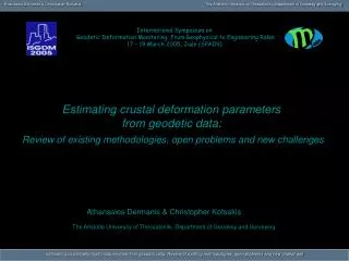
International Symposium on Geodetic Deformation Monitoring: From Geophysical to Engineering Roles 17 – 19 March 2005, Jaén (SPAIN) Estimating crustal deformation parameters from geodetic data: Review of existing methodologies, open problems and new challenges Athanasios Dermanis & Christopher Kotsakis The Aristotle University of Thessaloniki, Department of Geodesy and Surveying
International Symposium on Geodetic Deformation Monitoring: From Geophysical to Engineering Roles 17 – 19 March 2005, Jaén (SPAIN) Estimating crustal deformation parameters from geodetic data: Review of existing methodologies, open problems and new challenges Athanasios Dermanis & Christopher Kotsakis The Aristotle University of Thessaloniki Department of Geodesy and Surveying
THE ISSUES: What should be the end product of geodetic analysis? (Choice of parameters describing deformation) Which is the role of the chosen reference system(s)? 2-dimensional or 3-dimensional deformation? (Incorporating height variation information in a reasonable way) How should the necessary spatial (and/or temporal) interpolation be performed? (Trend removal and/or minimum norm interpolation) Data analysis strategy (Data coordinates / displacements deformation parameters) Quality assessment (effect of data errors and interpolation errors on final results)
An interplay between Geodesy and Geophysics: Crustal Deformation as an Inverse Problem y = Ax GEODESY GEOPHYSICS A acting forces geometric information (shape alteration) y equations of motion for deforming earth - - constitutional equations models for earth behavior (elasticity, viscocity,...) gravity variation information x density distribution hypotheses Geodetic product: Free of geophysical hypotheses!
An interplay between Geodesy and Geophysics: Crustal Deformation as an Inverse Problem y = Ax GEODESY GEOPHYSICS A acting forces geometric information (shape alteration) y equations of motion for deforming earth - - constitutional equations models for earth behavior (elasticity, viscocity,...) gravity variation information x density distribution hypotheses Geodetic product: Free of geophysical hypotheses!
The crustal deformation parameters to be produced by geodetic analysis
x0(λ) x(λ) x = f (x0) The deformation function f f O0 O Shape S0 Shape S
x0(λ) x(λ) The deformation gradient F x(λ) = f(x0(λ)) Two shapes of the same material curve parametric curve descriptions with parameter λ O O0 Shape S0 Shape S
x0(λ) dx0 dx x(λ) u0= u= dλ dλ The deformation gradient F tangent vectors to the curve shapes O O0 Shape S0 Shape S
x0(λ) x(λ) The deformation gradient F tangent vector length = rate of length variation ds0 ds |u0|= |u|= dλ dλ O O0 Shape S0 Shape S
x0(λ) u= F(u0) dx0 dx x(λ) u0= u= dλ dλ The deformation gradient F F O O0 Shape S0 Shape S
dxxdu0 = dλx0dλ x F= x0 The deformation gradient F Representation by a matrix F in chosen coordinate systems dx0 dx u0= u= dλ dλ F u= Fu0 x0(λ) x(λ) O0 O Shape S0 Shape S
Comparison of shapes at two epochs t0 and t space (coordinates) coordinate lines of material points time
Comparison of shapes at two epochs t0 and t x0=x(P,t0) x=x(P,t) space (coordinates) Observation of coordinates of all material points at 2 epochs: t0 and t Spatially continuous information time t0 t
Comparison of shapes at two epochs t0 and t x0 x Use initial coordinates as independent variables x0
Comparison of shapes at two epochs t0 and t x x Use coordinates at epoch t as dependent variables x0
Comparison of shapes at two epochs t0 and t x Deformation function f : x = f(x0 ) x0
f F(P) = (P) x0 Comparison of shapes at two epochs t0 and t x Deformation function f : x = f(x0 ) Deformation gradient F at point P = Local slope of deformation functionf : x0
f F(P) = (P) x0 Comparison of shapes at two epochs t0 and t x When only discrete spatial information is available We must perform spatial interpolation In order to compute the deformation gradient F x0
f F(P) = (P) x0 Comparison of shapes at two epochs t0 and t x When only discrete spatial information is available INTERPOLATION We must perform spatial interpolation In order to compute the deformation gradient F x0
SVD Singular Value Decomposition F = QT L P λ1 0 0 L = 0 λ2 0 0 0λ3 Physical interpretation of the deformation gradient From diagonalizations: C = U2 = FTF = PTL2P B = V2 = FFT = QTL2Q diagonal orthogonal Polar decomposition: F = QTLP = (QTP)(PTLP) = RU = (QTLQ) QTP = VR λ1, λ2, λ3 = singular values
F = QT L P e1(t) e2(t) e2(t0) Q R R P e1(t0) Physical interpretation of the deformation gradient SVD
F = QT L P e1(t) e2(t) e2(t0) e1(t0) Physical interpretation of the deformation gradient SVD This is all we can observe at the two epochs No relation of coordinate systems possible due to deformation
F = QT L P e1(t) e2(t0) e(t0) e(t) e2(t) e1(t0) The reference systems and cannot be identified in geodesy! We live on the deforming body and not in a rigid laboratory! Physical interpretation of the deformation gradient SVD Q R R P
R ~ ~ ~ Under x0 = S0x0, x = Sx : R = SRS0T ~ ~ S0,S inaccessible but common for all pointsR(x0) = SR(x0)S0T Local deformation F=QTLP consists of principal axes λ2 λ1 1 elongations L (scaling by λ1, λ2, λ3) along principal axes and a rotation R = QTP inaccessible in geodesy due to lack of coordinate system identification
e2(t0) e1(t0) Local deformation parameters (functions of F=QTLP ) principal axes R λ2 λ1 P 1 Singular values in L(λ1, λ2, λ3)and functions ψ(λ1,λ2,λ3) - Numerical invariants Angles in P(θ1, θ2, θ3)defining directions of principal axes (physical invariants) Angles in R(ω1, ω2, ω3)defining local rotation (not invariant)
e2(t0) e1(t0) Local deformation parameters (functions of F=QTLP ) principal axes R λ2 λ1 P 1 Singular values in L(λ1, λ2, λ3)and functions ψ(λ1,λ2,λ3) - Numerical invariants 2D 3D (areal) dilatation: Δ=λ1λ2-1 (volume) dilatation: Δ=λ1λ2λ3-1 shear: γ=(λ1-λ2) (λ1-λ2)-1/2 shears within principal planes: γik=(λi-λk) (λi-λk)-1/2 ik = 12, 23, 13
The role of the reference system
We need a reference system O(t), e1(t), e2(t), e3(t) for every epoch t ! (Dynamic or space-time reference system) Coordinates in an “preliminary” system, WGS 84, ITRF, or user defined: epoch t epoch t0 displacements too large !
m = ixi = const. (= 0) L2 = i ||xi – m||2 = const. 1 1 n n Definition of a network-intrinsic reference system: Center of mass preservation: hR = i [xi] vi = 0 Vanishing of relative angular momentum: Mean quadratic scale preservation:
Advantages of a network-intrinsic reference system: Invariant deformation parameters the same – No advantage for continuous spatial information Dermination of motion of the network area as whole: translation and rotation
Advantages of a network-intrinsic reference system: Invariant deformation parameters the same – No advantage for continuous spatial information Determination of motion of the network area as whole: translation & rotation Small displacements (trend removal): Essential for proper spatial interpolation of discrete spatial information Reference systems at 2 epochs identified
2-dimensional or 3-dimensional deformation?
Crustal deformation is a 3-dimensional physical process F t0 t
Usually studied as 2-dimensional by projection of physical surface to a “horizontal” plane F t0 t
Proper treatment: Deformation of the 2-dimensional physical surface as embedded in 3-dimensional space F t0 t
Attempts for a 3-dimensional treatment Extension of the 2D finite element method (triangular elements) to 3D (quadrilateral elements)
quadrilateral elements have much smaller vertical extension Attempts for a 3-dimensional treatment deformation of air ! We can obtain good horizontal information by interpolation or virtual densification. Vertical information requires extrapolation (an insecure process) deformation of mountain Derination of 3D crustal deformation from 2D deformation surface deformatiom (downward continuation) an improperly posed problem !
Spatial (and/or temporal) interpolation
Geodetic information on crustal deformation - Coordinates x(P,t) space The “ideal” situation: Space continuous Time continuous To provide deformation parameters at any point for any 2 epochs No interpolation needed ! time
Geodetic information on crustal deformation - Coordinates x(P,tk) space The “satisfactory” situation: Space continuous Time discrete To provide deformation parameters at any point for any 2 observation epochs No interpolation needed ! t1 t2 t3 t4 t5 t6 t7 time
Geodetic information on crustal deformation - Coordinates x(P,tk) space The “satisfactory” situation: Space continuous Time discrete To provide deformation parameters at any point for any 2 epochs Temporal interpolation needed ! t1 t2 t3 t4 t5 t6 t7 time
Geodetic information on crustal deformation - Coordinates x(Pi,tk) space The “realistic” situation: Space discrete Time discrete To provide deformation parameters at any point for any 2 observation epochs P6 P5 P4 P3 P2 Spatial interpolation needed ! P1 t1 t2 t3 t4 t5 t6 t7 time
Geodetic information on crustal deformation - Coordinates x(Pi,tk) space The “realistic” situation: Space discrete Time discrete To provide deformation parameters at any point for any 2 epochs P6 P5 P4 P3 P2 Spatial interpolation needed ! P1 Temporal interpolation also needed ! t1 t2 t3 t4 t5 t6 t7 time
Geodetic information on crustal deformation - Coordinates x(Pi,tk) Not all points observed at each epoch space The “realistic” situation: Space discrete Time discrete P6 P5 To provide deformation parameters at any point for any 2 observation epochs P4 P3 P2 Spatial interpolation needed ! P1 Temporal interpolation needed ! t1 t2 t3 t4 t5 t6 t7 time
Geodetic information on crustal deformation - Coordinates x(Pi,t) space GPS permanent stations Space discrete Time continuous To provide deformation parameters at any point for any 2 epochs P6 P5 P4 P3 P2 Spatial interpolation needed ! P1 t1 t2 t3 t4 t5 t6 t7 time
Geodetic information on crustal deformation - Coordinates x(Pi,t),x(Pi,tk) space GPS permanent stations and SAR interferometry Space discrete Time discrete (SAR) time - continuous (GPS) To provide deformation parameters at any point for any 2 SAR observation epochs P6 P5 P4 P3 P2 No spatial interpolation needed ! P1 t1 t2 t3 t4 t5 t6 t7 time
Geodetic information on crustal deformation - Coordinates x(Pi,t),x(Pi,tk) space GPS permanent stations and SAR interferometry Space discrete Time discrete (SAR) time - continuous (GPS) To provide deformation parameters at any point for any 2 epochs P6 P5 P4 P3 P2 Spatial interpolation needed ! P1 t1 t2 t3 t4 t5 t6 t7 time
Data analysis strategies