Advanced Ion Tracking in PRISMA: Optimizing Trajectories and Analysis Techniques
80 likes | 194 Views
This study focuses on the tracking of ions within the PRISMA facility at INFN, Padova. A detailed approach is discussed incorporating advanced algorithms for energy, time-of-flight, and position measurements using MCP, MWPPAC, and IC detectors. The methodology emphasizes a systematic mapping of magnetic fields and simplified transport equations to determine ion trajectories within the magnetic spectrometer. The iterative processes ensure accuracy while minimizing computational time, making this framework suitable for real-time applications. Experimental results validate the effectiveness of the new algorithms against historical data.

Advanced Ion Tracking in PRISMA: Optimizing Trajectories and Analysis Techniques
E N D
Presentation Transcript
Tracking ions inside PRISMA E.Farnea INFN Sezione di Padova
195 MeV 36S + 208Pb, lab = 80o Y Z=28 Dt ~ 350 ps, DX = 1 mm DY = 1 mm Y position DY = 2 mm E (a.u.) X Z=16 E (a.u.) X position Dt < 500 ps DX = 1 mm DE/E < 2% Z/DZ ~ 60 for Z=20 The PRISMA Magnetic Spectrometer MCP MWPPAC IC Q Dipole Z, A, b of the recoils through combination of: EnergyTOFDE-E Focal plane position Direction from the start detector E. Fioretto INFN - LNL E. Fioretto INFN - LNL
A possible approach In principle, once a detailed 3D map of the fields is known, the transportation through PRISMA is fully determined by the entrance position and by the magnetic rigidity: Where MD, MQ are called transportation matrices. In practice, high-order polynomial expansions are used (see eg A.Lazzaro, NIM A570, 192 (2007)) to invert the matrices and determine the trajectory of the ions.
The present approach In the case of PRISMA, we can take a simplified approach: Ideal magnetic elements are considered, reabsorbing fringe effects with a redefinition of the geometry (effective length) The trajectory from the dipole to the focal plane is essentially in the dispersion plane (~20cm vertical displacement vs ~400cm path) Given the size of the MCP start detector, the trajectories entering the quadrupole are essentially para-axial Once the magnetic rigidity of the ions is fixed, their motion is determined by the ratio of the magnetic fields, BD/BQ rather than their exact values In practice an iterative procedure is followed
The iterative procedure Transport to quadrupole(straight line) C++ and FORTRAN versions available Guess rigidity(curvature radius) Transport through quadrupole New guess rigidity Transport to dipole(straight line) No Focal plane coincides with observed? Transport through dipole(arc of circle) Yes Validate event with IC information
Results Original algorithm Present algorithm • The results with experimental PRISMA data are of the same quality as those obtained with the original algorithm used in GSORT • Few iterations per cycle are needed, fast enough for on-line (spy) implementation
The PRISMA presort library • User just needs to create an instance of a prismaManager object • prismaManager takes care of creating instances of other relevant objects • Experiment-specific configuration decoded from configuration files • User just asks for information to prismaManager, which will “forward the question to” the proper object • Data need to be formatted in a native format (not ADF, not yet available at the time of developing the library)
Implementation into Narval • Just completed, results soon to be seen …