Download
1 / 9
90 likes | 174 Views
Learn the terminology and parameters for aggregate production planning by linear programming. Understand decision variables and constraints in single-product models for efficient planning and optimization.

E N D
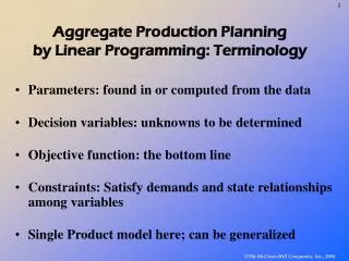
Aggregate Production Planning by Linear Programming: Terminology • Parameters: found in or computed from the data • Decision variables: unknowns to be determined • Objective function: the bottom line • Constraints: Satisfy demands and state relationships among variables • Single Product model here; can be generalized
Parameters: find these in the data! • dt = amount of product demanded in period t • pt = productivity per worker in period t • Lt = unit labor cost per worker in period t • ht = unit hiring cost per worker in period t • ft = unit firing cost per worker in period t
Parameters: find these in the data! • ct = inventory holding cost per unit per period in period t • at = backorder cost per item per period in period t
Decision Variables: find values by solving the model • wt = number of workers employed in period t • ut = number of workers hired between periods t-1 and t • vt = number of workers fired between periods t-1 and t • it = amount of product in inventory at the end of period t • bt = amount backordered at the end of period t
Initial values: “fixed variables”; find in data • io = initial inventory level • wo = initial workforce level
The LP Model Minimize t (Ltwt + htut + ftvt + ctit + atbt) s.t. ut - vt = wt – wt-1 for each period t : workforce change ptwt + it-1 - it + bt – bt-1 = dt for each period t: demand balance wt, ut, vt, it, bt 0 for each time period t: nonnegativity
The LP Model Minimize t (128wt + 500ut + 1000vt + 10it + 100bt) s.t. u1 – v1 = w1 – w0 : workforce change, period 1,… 26.67wt + io – i1 + b1 – bo = dt: demand balance, period 1… wt, ut, vt, it, bt 0 for each time period t: nonnegativity