An Algorithm for the Steiner Problem in Graphs
730 likes | 910 Views
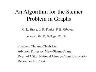
An Algorithm for the Steiner Problem in Graphs. M. L. Shore, L. R. Foulds, P. B. Gibbons. Networks, Vol. 12, 1982, pp. 323-333. Speaker: Chuang-Chieh Lin Advisor: Professor Maw-Shang Chang Dept. of CSIE, National Chung-Cheng University December 10, 2004. Outline. Introduction

An Algorithm for the Steiner Problem in Graphs
E N D
Presentation Transcript
An Algorithm for the Steiner Problem in Graphs M. L. Shore, L. R. Foulds, P. B. Gibbons Networks, Vol. 12, 1982, pp. 323-333. Speaker: Chuang-Chieh Lin Advisor: Professor Maw-Shang Chang Dept. of CSIE, National Chung-Cheng University December 10, 2004
Outline • Introduction • Related works • Branch-and-bound strategy • General concept of the algorithm • The branching method • The bounding method • Numerical example • Conclusion • References Dept. of CSIE, CCU, Taiwan
Outline • Introduction • Related works • Branch-and-bound strategy • General concept of the algorithm • The branching method • The bounding method • Numerical example • Conclusion • References Dept. of CSIE, CCU, Taiwan
Introduction Jakob Steiner • Steiner’s problem (SP) • SP is concerned with connecting a given set of points in an Euclidean plane by lines in the sense that there is a path of lines between every pair in the set. • Steiner problem in graphs (SPG) • SPG is a graph-theoretic version of the SP. • Let G be a graph denoted by an ordered pair (V, E), where V is the set of points and E is a set of undirected edges jointing pairs of distinct points of V. Dept. of CSIE, CCU, Taiwan
SPG (contd.) • Let w : E→R be a weight function, such that each edge e in E has a weight w(e), where R is the set of real numbers. For each edge eij = {vi, vj} in E, we denote its weight w(eij) by wij. • A path between point vi and vj in G is a sequence of the form: where vαk, k = 1, 2, …, p, are distinct points in G and the pairs are edges in G. Dept. of CSIE, CCU, Taiwan
SPG (contd.) • SPG is then defined as follows: • Given a weighted graph G = (V, E) and a nonempty subset V' of V, the SPG requires the identification of a subset E* of E such that: • The edges in E* connect the points in V' in the sense that between every pair of points in V', there exists a path comprising only edges in E*. • The sum of weights of the edges in E* is a minimum. Dept. of CSIE, CCU, Taiwan
SPG (contd.) • To discuss this article more conveniently, we call the vertices in V'terminals, and vertices in V\V'Steiner points from now on. • Throughout discussing this article, we assume that all edges of any graph G = (V, E) under consideration have non-negative weight. Dept. of CSIE, CCU, Taiwan
This restriction means that among the optimal solutions, there will exist a tree. • Thus we shall solve the SPG by finding a tree containing V' which is a subgraph of G and is of minimum total weight. • Let us see some examples. Dept. of CSIE, CCU, Taiwan
5 A Steiner tree 6 5 2 2 2 3 4 3 2 2 4 13 : E\E* : E* : V' ; terminals : V/V' ; Steiner points The sum of weights of this Steiner tree is 2+2+2+2+4=12. Dept. of CSIE, CCU, Taiwan
5 Another Steiner tree 6 5 2 2 2 3 4 3 2 2 4 13 : E\E* : E* : V' ; terminals : V /V' ; Steiner points The sum of weights of this Steiner tree is 4+2+2+3+4=15. Dept. of CSIE, CCU, Taiwan
Special cases: • |V'| = 1: single point => The optimal solution has no edges and zero total weight. • |V'| = 2: SPG can be reduced to finding the shortest path in G between the nodes in V '. • |V'| = |V|: SPG can be reduced to the minimal spanning tree problem. Dept. of CSIE, CCU, Taiwan
Outline • Introduction • Related works • Branch-and-bound strategy • General concept of the algorithm • The branching method • The bounding method • Numerical example • Conclusion • References Dept. of CSIE, CCU, Taiwan
Related works • Melzak [M61] and Cockayne [C70] have given exact algorithms for the SP respectively. (Only small SP’s can be handled by these algorithms) • Chang [C72] and Scott [S71] proposed heuristics for larger SP’s. • For the special case of constructing a Steiner tree with a given topology, Hakimi [H71] proposed an algorithm based on the method of Melzakfor the SP. Dept. of CSIE, CCU, Taiwan
Related works (contd.) • Hakimi [H71] examined the general SPG and provided an algorithm for its solution. Hakimi also showed that a solution to the SPG also yields solutions to the problems of finding a maximum independent set and a minimum dominating set. • Dreyfus and Wagner [DW72] presented an algorithm for the general SPG which is similar in spirit to dynamic programming and requires the calculation of the shortest path between every pair of points in the graph. Dept. of CSIE, CCU, Taiwan
Related works (contd.) • According to Christofides [C72a], these algorithms above are not bad in experimental results but they can’t handle problems with much above 10 points in V' in reasonable computing time. • Takahashi and Matsuyama [TM80] have presented an algorithm based on Dijkstra’s minimal spanning tree algorithm, which finds an approximate solution in (kn2) time, where k = |V'| and n = |V|. The worse case cost ratio of the obtained solution to the optimal solution is tightly 2(1 1/k). Dept. of CSIE, CCU, Taiwan
Outline • Introduction • Related works • Branch-and-bound strategy • General concept of the algorithm • The branching method • The bounding method • Numerical example • Conclusion • References Dept. of CSIE, CCU, Taiwan
Branch-and-bound strategy • The general ideas: • Each edge eij can be temporarily excluded from consideration. • The set of included edges for a partial solution will form a set of connected components; those components that contain points in V' are calledessential components. • The criterion for a solution to be feasible is that there is only one essential component. (All points in V' are connected by the set of includes edges.) include exclude Dept. of CSIE, CCU, Taiwan
As an edge eij is added to the set of included edges, the components containing vi an vj will be combined to form one component. • When a further edge is excluded, the component structure remains unaltered. • The algorithm is as follows: Dept. of CSIE, CCU, Taiwan
The algorithm: • <1> Let |V| = n and |V'| = m. Relabel the points in V' as v1, v2, , vm and those in V \V' as vm+1, vm+2,, vn. • <2>Construct a matrix W = [wij]nn, where Dept. of CSIE, CCU, Taiwan
<3>Calculate the lower bound and upper bound at this node. • (Fathomed) If the lower bound is equal to the upper bound, return the feasible solution. • (Fathomed) If the lower bound is greater than the presently found lowest upper bound, discard this node. • (Fathomed) If the node itself represents an infeasible solution, discard this node. Dept. of CSIE, CCU, Taiwan
(Unfathomed) Else, branch on each node to two nodes. One node is generated by excluding an edge from consideration and the other one is generated by including it in the partial solution. The latter node is always selected first. (This leads to an initial examination of successive partial solutions of accepted edges.) => < depth-first > • <4> Backtrack the partial solutions then: • the optimal solution is uncovered • or the evidence that no such solution exists is provided. • Next, let us proceed to the branching method. Dept. of CSIE, CCU, Taiwan
Outline • Introduction • Related works • Branch-and-bound strategy • General concept of the algorithm • The branching method • The bounding method • Numerical example • Conclusion • References Dept. of CSIE, CCU, Taiwan
The branching method • Assume that we are branching on an unfathomed node N. • We associate with each edge a penalty for not adding it to the set of included edges. • The edge with the largest penalty will be selected for branching. • How do we calculate a penalty? • penalty vector Dept. of CSIE, CCU, Taiwan
A penalty vector T = {ti: i = 1, 2, , m} is calculated as follows: • Compute ki = the value of j producing wi*. • Compute . • Compute • At last, Then the edge er, kr is the edge to branch. Two nodes emanating from N are created. It is some kind of heuristic idea! Dept. of CSIE, CCU, Taiwan
v1 v3 5 5 v2 5 5 4 4 4 v4 4 v5 (v1, v2, v3, v4 are terminals and v5 is a Steiner point.) • For example, let us see the following graph: tr = 1 and the edge to branch can bee1, 5 Dept. of CSIE, CCU, Taiwan
v1 v3 v2 v4 v5 v1 v1 v3 v3 v2 v2 4 v4 v4 v5 v5 Node 1 Node 2 Node 0 or Dept. of CSIE, CCU, Taiwan
In order to produce a bound for a new partial solution, we must temporarily adjust the weight matrix W. • If the new partial solution was produced by adding exy to the set of excluded edges, then we temporarily set wxy = wyx = ∞. • If the new partial solution was produced by adding exy to the set of included edges, then components, cx and cy, where vx and vy belong are combined. W is then transformed to W' with one less row in each row and one less column in each column. Dept. of CSIE, CCU, Taiwan
<for included edges> • Thus if we let W' =[w'ij], • If 1 ≤ x ≤ m, • Otherwise, (x’s are terminals) (x’s are Steiner points) Dept. of CSIE, CCU, Taiwan
For example, in the previous example, At node 1, W will be temporarily changed to v1 and v5 are combined Dept. of CSIE, CCU, Taiwan
At node 2, W will be temporarily changed to Dept. of CSIE, CCU, Taiwan
Outline • Introduction • Related works • Branch-and-bound strategy • General concept of the algorithm • The branching method • The bounding method • Numerical example • Conclusion • References Dept. of CSIE, CCU, Taiwan
The bounding method • Upper bound: • At each branching node N, finding the minimal spanning tree from the current node. Then the sum of weights of this tree is an upper bound for N. (Actually, The authors didn’t calculate the upper bounds, so we omit the proof here.) • Lower bound: • The Lower bound is calculated for a node with weight matrix Wby using the following theorem. Dept. of CSIE, CCU, Taiwan
The bounding method (contd.) • Theorem. Consider an SPG on graph G = (V, E) with the optimal solution z*. Then we have z* min{b, c}, where Dept. of CSIE, CCU, Taiwan
Proof: • Consider a minimal tree T* with length z* spanning V'. • Suppose T* = (V*, E*), where V' V* V and E* E. • T* can be represented as the ordered triple (Vt, E*, vt), where Vt {vt} = V*, and there is a one-to-one correspondence h: Vt→ E* such that vi is incident with h(vi), for all viVt. • Now, let us discuss about the following two cases: • Case I: V*\V' • Case II: V*= V'. Think about the reason ! Dept. of CSIE, CCU, Taiwan
Case I. V*\V' , i.e., k, m < k ≤ ns.t. vk V*\V'. • Let vt = vk. Therefore V' Vt as vk V'. • Thus since E* E. Dept. of CSIE, CCU, Taiwan
V* contains only terminals, T* becomes the minimal spanning tree of V*, that is, V'. • Case II. V*= V'. • Given any vtV*, {h(vi): viVt} = E*. Let • Let vt = vg. Now, vd vg = vt Dept. of CSIE, CCU, Taiwan
(Note that {h(vi): viVt} = E*.) since Vt{vt} = V* = V' and vt = vg since E* V*V* = V' V' Therefore, we have shown that z* b or z* c. ■ Dept. of CSIE, CCU, Taiwan
Outline • Introduction • Related works • Branch-and-bound strategy • General concept of the algorithm • The branching method • The bounding method • Numerical example • Conclusion • References Dept. of CSIE, CCU, Taiwan
6 4 1 7 5 3 2 Numerical example • Now, let us see an example. m = 4 Dept. of CSIE, CCU, Taiwan
Node 1 (4) ~ e4,5 e4,5 The authors’ decision tree nodes Node 2 (4) Node 17 (7) ~ e5,7 e5,7 discard Node i (lower bound) Node16 (7) Node 3 (5) ~ e1,7 e1,7 discard node Node15 (7) Node 4 (6) e6,7 ~ e6,7 discard Node 5 (7) ~ e3,7 Node 10 (6) e3,7 ~ e2,3 Node 9 (7) Node 6 (7) e2,3 Node 14 (7) ~ e2,3 e2,3 discard discard Node 8 (∞) Node 7 (7) Node 11 (6) ~ e3,7 e3,7 discard solution Node 13 (∞) Node 12 (6) solution discard Dept. of CSIE, CCU, Taiwan
Node 1 (4, ∞) My decision tree nodes ~ e4,5 e4,5 Node 7 (7, 6) Node 2 (4, 7) Node i (lower bound, upper bound) ~ e5,7 e5,7 discard Node 6 (7, 6) Node 3 (5, 6) node ~ e1,7 e1,7 discard Node 5 (7, 6) Node 4 (6, 6) discard solution Next, we will concentrate on this bounding procedure. Dept. of CSIE, CCU, Taiwan
Node 1: <> b = 1 + 1 + 1 + 1 = 4; c = (2 + 1 + 1 + 4) (1) = 7 • lower bound = min {b, c} = 4 • upper bound = ∞ global upper bound (by finding a minimal spanning tree of v1, v2, v3 and v4) pick? Dept. of CSIE, CCU, Taiwan
~ e4,5 e4,5 Node 7 (?, ?) Node 2 (?, ?) Node 1 (4,∞) Dept. of CSIE, CCU, Taiwan
For node 2: (pick e4, 5) For node 7: (don’t pick e4, 5) Dept. of CSIE, CCU, Taiwan
Node 2: < e4,5 > b =1+1+1+1=4; c=(2+1+1+1)(1) =4 • lower bound = 1+min {b, c} = 5 • upper bound = |e4, 5|+| e5, 1|+|e1, 2|+|e2, 3|=1+3+2+1=7 global upper bound (by finding a minimal spanning tree of v1, v2, v3 and v4-5) pick? Dept. of CSIE, CCU, Taiwan
~ e5,7 e5,7 Node 6 (?, ?) Node 3 (?, ?) Node 1 (4, ∞) ~ e4,5 e4,5 Node 7 (?, ?) Node 2 (4,7) Dept. of CSIE, CCU, Taiwan
For node 3: (picke5,7) For node 6: (don’t picke5,7) Dept. of CSIE, CCU, Taiwan
Node 3:< e4,5 ,e5,7 > b =1+1+1+1=4; c=(1+1+1+1)(1) =3 • lower bound = 2 + min {b, c} = 5 • upper bound = |e4,5|+| e5,7|+|e7,1|+|e1,2|+|e2,3|=1+1+1+2+1=6 global upper bound (by finding a minimal spanning tree of v1, v2, v3 and v4-5-7) pick? Dept. of CSIE, CCU, Taiwan
~ e1,7 e1,7 Node 5 (?, ?) Node 4 (?, ?) Node 1 (4, ∞) ~ e4,5 e4,5 Node 7 (?, ?) Node 2 (4, 7) ~ e5,7 e5,7 Node 6 (?, ?) Node 3 (5, 6) Dept. of CSIE, CCU, Taiwan
For node 4: (picke1,7) For node 5: (don’t picke1,7) Dept. of CSIE, CCU, Taiwan