Download
1 / 58
580 likes | 744 Views
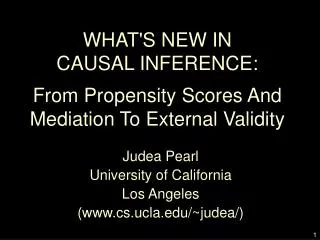
WHAT'S NEW IN CAUSAL INFERENCE: From Propensity Scores And Mediation To External Validity. Judea Pearl University of California Los Angeles (www.cs.ucla.edu/~judea/). OUTLINE. Unified conceptualization of counterfactuals, structural-equations, and graphs Propensity scores demystified

E N D
WHAT'S NEW IN CAUSAL INFERENCE: From Propensity Scores And Mediation To External Validity Judea Pearl University of California Los Angeles (www.cs.ucla.edu/~judea/)
OUTLINE • Unified conceptualization of counterfactuals, structural-equations, and graphs • Propensity scores demystified • Direct and indirect effects (Mediation) • External validity mathematized
P Joint Distribution Q(P) (Aspects of P) Data Inference TRADITIONAL STATISTICAL INFERENCE PARADIGM e.g., Infer whether customers who bought product A would also buy product B. Q = P(B | A)
THE STRUCTURAL MODEL PARADIGM Joint Distribution Data Generating Model Q(M) (Aspects of M) Data M Inference • M – Invariant strategy (mechanism, recipe, law, protocol) by which Nature assigns values to variables in the analysis. “Think Nature, not experiment!”
FAMILIAR CAUSAL MODEL ORACLE FOR MANIPILATION X Y Z INPUT OUTPUT
e.g., STRUCTURAL CAUSAL MODELS • Definition: A structural causal model is a 4-tuple • V,U, F, P(u), where • V = {V1,...,Vn} are endogeneas variables • U={U1,...,Um} are background variables • F = {f1,...,fn} are functions determining V, • vi = fi(v, u) • P(u) is a distribution over U • P(u) and F induce a distribution P(v) over observable variables
The Fundamental Equation of Counterfactuals: CAUSAL MODELS AND COUNTERFACTUALS Definition: The sentence: “Y would be y (in situation u), had X beenx,” denoted Yx(u) = y, means: The solution for Y in a mutilated model Mx, (i.e., the equations for X replaced by X = x) with input U=u, is equal to y.
READING COUNTERFACTUALS FROM SEM Data shows: a = 0.7, b = 0.5, g = 0.4 A student named Joe, measured X=0.5, Z=1, Y=1.9 Q1: What would Joe’s score be had he doubled his study time?
READING COUNTERFACTUALS Q1: What would Joe’s score be had he doubled his study time? Answer: Joe’s score would be 1.9 Or, In counterfactual notaion:
READING COUNTERFACTUALS Q2: What would Joe’s score be, had the treatment been 0 and had he studied at whatever level he would have studied had the treatment been 1?
Joint probabilities of counterfactuals: In particular: CAUSAL MODELS AND COUNTERFACTUALS Definition: The sentence: “Y would be y (in situation u), had X beenx,” denoted Yx(u) = y, means: The solution for Y in a mutilated model Mx, (i.e., the equations for X replaced by X = x) with input U=u, is equal to y.
THE FIVE NECESSARY STEPS OF CAUSAL ANALYSIS Define: Assume: Identify: Estimate: Test: Express the target quantity Q as a function Q(M) that can be computed from any model M. Formulate causal assumptions Ausing some formal language. Determine if Q is identifiable given A. EstimateQ if it is identifiable; approximate it, if it is not. Test the testable implications of A (if any).
THE LOGIC OF CAUSAL ANALYSIS CAUSAL MODEL (MA) CAUSAL MODEL (MA) A - CAUSAL ASSUMPTIONS A* - Logical implications of A Causal inference Q Queries of interest Q(P) - Identified estimands T(MA) - Testable implications Statistical inference Data (D) Q - Estimates of Q(P) Goodness of fit Provisional claims Model testing
G IDENTIFICATION IN SCM Find the effect ofXonY, P(y|do(x)), given the causal assumptions shown inG, whereZ1,..., Zk are auxiliary variables. Z1 Z2 Z3 Z4 Z5 X Z6 Y CanP(y|do(x))be estimated if only a subset,Z, can be measured?
G Gx Moreover, (“adjusting” for Z) Ignorability ELIMINATING CONFOUNDING BIAS THE BACK-DOOR CRITERION P(y | do(x)) is estimable if there is a set Z of variables such thatZd-separates X from YinGx. Z1 Z1 Z2 Z2 Z Z3 Z3 Z4 Z5 Z5 Z4 X X Z6 Y Y Z6
Watch out! No, no! EFFECT OF WARM-UP ON INJURY (After Shrier & Platt, 2008) ??? Front Door Warm-up Exercises (X) Injury (Y)
L Theorem: Adjustment for L replaces Adjustment for Z PROPENSITY SCORE ESTIMATOR (Rosenbaum & Rubin, 1983) Z1 Z2 P(y | do(x)) = ? Z4 Z3 Z5 X Z6 Y Can L replace {Z1, Z2, Z3, Z4, Z5} ?
Z Z Z X Y X Y X Y X Y WHAT PROPENSITY SCORE (PS) PRACTITIONERS NEED TO KNOW • The asymptotic bias of PS is EQUAL to that of ordinary adjustment (for same Z). • Including an additional covariate in the analysis CANSPOIL the bias-reduction potential of others. Z • In particular, instrumental variables tend to amplify bias. • Choosing sufficient set for PS, requires knowledge of the model.
SURPRISING RESULT: Instrumental variables are Bias-Amplifiers in linear models (Bhattarcharya & Vogt 2007; Wooldridge 2009) (Unobserved) Z U c3 c1 c2 X Y c0 “Naive” bias Adjusted bias
Z Z U U c3 c3 c1 c1 c2 c2 X X Y Y c0 c0 INTUTION: When Z is allowed to vary, it absorbs (or explains) some of the changes in X. When Z is fixed the burden falls on U alone, and transmitted to Y (resulting in a higher bias) Z U c3 c1 c2 X Y c0
WHAT’S BETWEEN AN INSTRUMENT AND A CONFOUNDER? Should we adjust for Z? U Z c4 c1 c3 c2 T1 T2 c0 Y X Yes, if No, otherwise Adjusting for a parent of Y is safer than a parent of X ANSWER: CONCLUSION:
Z T X Y WHICH SET TO ADJUST FOR Should we adjust for {T},{Z}, or {T, Z}? Answer 1: (From bias-amplification considerations) {T} is better than {T, Z} which is the same as {Z} Answer 2: (From variance considerations) {T} is better than {T, Z} which is better than {Z}
CONCLUSIONS • The prevailing practice of adjusting for all covariates, especially those that are good predictors of X(the “treatment assignment,” Rubin, 2009) is totally misguided. • The “outcome mechanism” is as important, and much safer, from both bias and variance viewpoints • As X-rays are to the surgeon, graphs are for causation
The mothers of all questions: Q. When would b equal a? A. When all back-door paths are blocked, (uY X) REGRESSION VS. STRUCTURAL EQUATIONS (THE CONFUSION OF THE CENTURY) Regression (claimless, nonfalsifiable): Y = ax + Y Structural (empirical, falsifiable): Y = bx + uY Claim: (regardless of distributions): E(Y | do(x)) = E(Y | do(x), do(z)) = bx Q. When is b estimable by regression methods? A. Graphical criteria available
TWO PARADIGMS FOR CAUSAL INFERENCE Observed: P(X, Y, Z,...) Conclusions needed: P(Yx=y), P(Xy=x | Z=z)... How do we connect observables, X,Y,Z,… to counterfactuals Yx, Xz, Zy,… ? N-R model Counterfactuals are primitives, new variables Super-distribution Structural model Counterfactuals are derived quantities Subscripts modify the model and distribution
inconsistency: x = 0 Yx=0 = Y Y = xY1 + (1-x) Y0 “SUPER” DISTRIBUTION IN N-R MODEL X 0 0 0 1 Y 0 1 0 0 Z 0 1 0 0 Yx=0 0 1 1 1 Yx=1 1 0 0 0 Xz=0 0 1 0 0 Xz=1 0 0 1 1 Xy=0 0 1 1 0 U u1 u2 u3 u4
ARE THE TWO PARADIGMS EQUIVALENT? • Yes (Galles and Pearl, 1998; Halpern 1998) • In the N-R paradigm, Yx is defined by consistency: • In SCM, consistency is a theorem. • Moreover, a theorem in one approach is a theorem in the other. • Difference: Clarity of assumptions and their implications
AXIOMS OF STRUCTURAL COUNTERFACTUALS Yx(u)=y: Ywould bey, hadXbeenx(in stateU = u) (Galles, Pearl, Halpern, 1998): • Definiteness • Uniqueness • Effectiveness • Composition (generalized consistency) • Reversibility
1. English: Smoking (X), Cancer (Y), Tar (Z), Genotypes (U) U Y X Z 2. Counterfactuals: 3. Structural: Z X Y FORMULATING ASSUMPTIONS THREE LANGUAGES
COMPARISON BETWEEN THE N-R AND SCM LANGUAGES • Expressing scientific knowledge • Recognizing the testable implications of one's assumptions • Locating instrumental variables in a system of equations • Deciding if two models are equivalent or nested • Deciding if two counterfactuals are independent given another • Algebraic derivations of identifiable estimands
GRAPHICAL – COUNTERFACTUALS SYMBIOSIS Every causal graph expresses counterfactuals assumptions, e.g., X Y Z • Missing arrows Y Z 2. Missing arcs Y Z • consistent, and readable from the graph. • Express assumption in graphs • Derive estimands by graphical or algebraic methods
EFFECT DECOMPOSITION (direct vs. indirect effects) • Why decompose effects? • What is the definition of direct and indirect effects? • What are the policy implications of direct and indirect effects? • When can direct and indirect effect be estimated consistently from experimental and nonexperimental data?
WHY DECOMPOSE EFFECTS? • To understand how Nature works • To comply with legal requirements • To predict the effects of new type of interventions: • Signal routing, rather than variable fixing
LEGAL IMPLICATIONS • OF DIRECT EFFECT Can data prove an employer guilty of hiring discrimination? X Z (Gender) (Qualifications) Y (Hiring) What is the direct effect of X on Y ? (averaged over z) Adjust for Z? No! No!
FISHER’S GRAVE MISTAKE • (after Rubin, 2005) What is the direct effect of treatment on yield? X Z (Soil treatment) (Plant density) (Latent factor) Y (Yield) Compare treated and untreated lots of same density No! No! Proposed solution (?): “Principal strata”
NATURAL INTERPRETATION OF AVERAGE DIRECT EFFECTS Robins and Greenland (1992) – “Pure” X Z z = f (x, u) y = g (x, z, u) Y Natural Direct Effect of X on Y: The expected change in Y, when we change X from x0 to x1 and, for each u, we keep Z constant at whatever value it attained before the change. In linear models, DE = Natural Direct Effect
DEFINITION AND IDENTIFICATION OF NESTED COUNTERFACTUALS Consider the quantity Given M, P(u), Q is well defined Given u,Zx*(u) is the solution for Z in Mx*,call it z is the solution for Y in Mxz Can Q be estimated from data? Experimental: nest-free expression Nonexperimental: subscript-free expression
DEFINITION OF INDIRECT EFFECTS X Z z = f (x, u) y = g (x, z, u) No Controlled Indirect Effect Y Indirect Effect of X on Y: The expected change in Y when we keep Xconstant, say at x0, and let Zchange to whatever value it would have attained had X changed to x1. In linear models, IE = TE - DE
GENDER QUALIFICATION HIRING POLICY IMPLICATIONS OF INDIRECT EFFECTS What is the indirect effect of X on Y? The effect of Gender on Hiring if sex discrimination is eliminated. X Z IGNORE f Y Deactivating a link – a new type of intervention
MEDIATION FORMULAS • The natural direct and indirect effects are identifiable in Markovian models (no confounding), • And are given by: • Applicable to linear and non-linear models, continuous and discrete variables, regardless of distributional form.
g xz Linear + interaction Z m1 m2 X Y In linear systems
Z X Y MEDIATION FORMULAS IN UNCONFOUNDED MODELS
TE TE - DE IE DE Disabling direct path Disabling mediation Z m1 m2 X Y In linear systems Is NOT equal to:
Z MEDIATION FORMULA FOR BINARY VARIABLES X Y
RAMIFICATION OF THE MEDIATION FORMULA • DE should be averaged over mediator levels, • IE should NOT be averaged over exposure levels. • TE-DE need not equal IE • TE-DE = proportion for whom mediation is necessary • IE = proportion for whom mediation is sufficient • TE-DE informs interventions on indirect pathways • IE informs intervention on direct pathways.
Z = age Z = age Y Y X X TRANSPORTABILITY -- WHEN CAN WE EXTRPOLATE EXPERIMENTAL FINDINGS TO DIFFERENT POPULATIONS? Experimental study in LA Measured: Problem: We find (LA population is younger) What can we say about Intuition: Observational study in NYC Measured:
Z Z Y Y X X Z Y X (b) (a) (c) TRANSPORT FORMULAS DEPEND ON THE STORY a) Z represents age b) Z represents language skill c) Z represents a bio-marker
TRANSPORTABILITY (Pearl and Bareinboim, 2010) • Definition 1 (Transportability) • Given two populations, denoted and *, • characterized by models M = <F,V,U>and • M* = <F,V,U+S>, respectively, a causal relation • R is said to be transportable from to * if • 1. R() is estimable from the set I of interventional studies on , and • 2. R(*) is identified from I, P*, G, and G + S. S = external factors responsible for MM*
S S Z S Z Y Y X X Z Y X (b) (a) (c) TRANSPORT FORMULAS DEPEND ON THE STORY a) Z represents age b) Z represents language skill c) Z represents a bio-marker ? ?
WHICH MODEL LICENSES THE TRANSPORT OF THE CAUSAL EFFECT S S S X Y X Y X Z Y (a) (b) (c) S S S X W Z Y X X Z Z Y Y (d) (f) ( S S S X X X W W W Z Z Z Y Y Y (e)