Download
1 / 26
260 likes | 380 Views
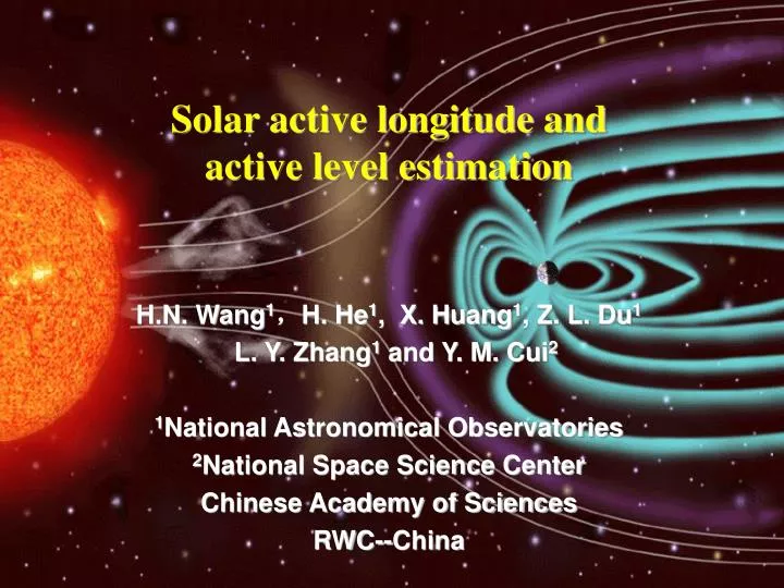
H.N. Wang 1 , H. He 1 , X. Huang 1 , Z. L. Du 1 L. Y. Zhang 1 and Y. M. Cui 2 1 National Astronomical Observatories 2 National Space Science Center Chinese Academy of Sciences RWC--China. Solar active longitude and active level estimation. Outline

E N D
H.N. Wang1,H. He1, X. Huang1, Z. L. Du1 L. Y. Zhang1 and Y. M. Cui2 1National Astronomical Observatories 2National Space Science Center Chinese Academy of Sciences RWC--China Solar active longitude and active level estimation
Outline • Solar Active Longitudes • Where solar activity often occurs • Solar Activity Level Estimation • How to estimate activity level of active regions • Summy
1. Solar Active Longitudes (1) Two persistent active longitudes of sunspots (Usoskin, et al., 2005, A&A, 441, 347 ) The distribution of sunspots is non-axisymmetric implies that the existence of two persistent (on century scale) active longitudes separated by 180 deg. These longitudes migrate with differential rotation and periodically alternate their activity levels showing a flip-flop cycle.
The longitudinal distribution of the sunspot area during cycle No. 19.(Usoskin, et al., 2005, A&A, 441, 347 ) The expected migration path of the two active longitudes according to differential rotation law
The corrected longitudinal distribution of the sunspot area during cycle No. 19.(Usoskin, et al., 2005, A&A, 441, 347 ) The longitudinal distribution of the sunspot area is corrected with a dynamic reference frame based on differential rotation law
Longitudinal distributions of sunspot occurrence in the Northern hemisphere for the period 1878--1996. a) Actual sunspots (area weighted) in the Carrington frame. The distribution is nearly isotropic. b) The same as panel a) but in the dynamic reference frame. c) Only the position of one dominant spot for each Carrington rotation is considered. d) The same as in panel c) but for 6-months averages. (Usoskin, et al , 2005, A&A, 441, 347)
(2) Two persistent active longitudes of solar X-ray flares (Zhang, et al 2007, A&A, 471, 711 ) When the Usoskins’s method was employed for observational solar flare data, the same phenomenon was found in the longitudinal distribution of powerful X-ray flares.
a) Data Optical flares associated with all the solar X-ray flares ≥ C class observed by GOES during the period of 1975 to 2005; Sunspots collected at the Royal Greenwich Observatory, the US Air Force, and NOAA for the same period as X-ray flares. b) Analysis Method The longitudinal distribution of the solar flares is corrected with a dynamic reference frame based on differential rotation law.
c) Result The observed longitude distribution of X-Class flares in the Carrington frame for the period of 1975–2005 The revised longitude distribution of X-class flares by differential rotation law
Non-axisymmetry comparison between flare and sunspot number This fact means that active longitudes related to X-ray flare location are more outstanding than those related to sunspot location.
(3) Application: X-ray flares in 23rd solar cycle • Nf the number of flares occurred in longitudes with h width • Nt the total number of all flares
2. Solar Activity Level Estimation (1) Solar flare productivity Solar active strength GOES X-ray flux is employed as a quantitative parameter for describing solar active strength Active sample A sample with GOES X-ray flux is larger than a threshold is called active sample
Forecasting time window A forward looking period when a parameter is measured at a moment. Flare productivity P(x) = Sa(x)/St(x), where X is a random value of measures describing magnetic properties, Sa(X) and St(X) are the number of the active samples and that of the total when values of these parameters are in the range [X,∞], respectively.
(2) Statistical analyses Data (1996-2006) MDI/SOHO manetograms : 23990 related active regions : 839 HSOS vector magnetograms: 1353 related active regions : 554 near the central of solar disk(E30o-W30o). Threshold for total soft X-ray flux: to be equivalent to a M1 flare
Selected parameters Maximum of horizontal gradient in longitudinal field |hBz|m length of neutral line with high horizontal gradient L number of singular points in transverse field
Solar flare productivity and magnetic measures (Cui, Y. M. et al , 2006, 2007; Wang, H. N. et al, 2009;Yu D. R. et al, 2010)
A1 and A2 are two asymptotic values • W is approximate width between these two asymptotic values • X0 is the center of W 2014/6/7 20 Dimensionless parameter
(3) Modeling and validation 1-Nearest Neighbor Model
Validation • Hit rate not considering active longitudes ~0.7 • correct rejection rate not considering active longitudes ~ 0.7 • Hit rate not considering active longitudes ~0.75 • correct rejection rate not considering active longitudes ~ 0.75
Summary • Active longitude can be predicted by considering the solar surface differential rotation (Zhang, et al 2007, 2011) • Activity level of active regions can be estimated by the dimensionless method (Wang, et al 2009) • Combination between active longitudes and active level estimation will be beneficial to modeling for solar activity forecasting.
For all of these measures, we have sigmoid function fittings : were Y is the flare productivity, and X is the value of measures.