Graph Theory
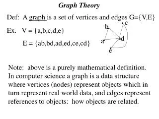
Graph Theory. Arnold Mesa. Basic Concepts. A graph G = (V,E) is defined by a set of vertices and edges. Edge (e1). Vertex (v1). v2. v1. v3. A Graph with 3 vertices and 3 edges. Basic Concepts (cont.).

Graph Theory
E N D
Presentation Transcript
Graph Theory Arnold Mesa
Basic Concepts • A graph G = (V,E) is defined by a set of vertices and edges Edge (e1) Vertex (v1) v2 v1 v3 A Graph with 3 vertices and 3 edges
Basic Concepts (cont.) • A vertex (v1) is said to be adjacent to (v2) if and only if they share a common edge (e1). e1 e2 v1 v2 v3
Basic Concepts (cont.) • A directed graph or digraph is a graph where direction matters. • Movement in the graph is determined by the direction of the edge. v2 v3 v1 v4 v6 v5
Basic Concepts (cont.) • A path in a graph is a sequence of vertices (v1, v2, v3,…,vn). • The path length is determined by how many edges are on the path. 2 v2 v3 1 3 v1 v4 v6 v5
Adjacency List Representation v2 v3 v1 v4 v6 v5 v1 v2 v2 v3 v6 v3 v4 v6 v4 v3 v5 v5 v6 v6 v1 Bi-Directional paths are allowed
More terms… • An edge may have a component known as a weight or cost associated to it. 4 6 v1 v2 v3
Adjacency Matrix Representation 1 v2 v3 6 6 4 3 6 v1 v4 4 7 v6 v5 4 v1 v2 v3 v4 v5 v6 v1 0 6 0 0 0 0 v2 0 0 1 0 0 4 v3 0 0 0 6 5 3 v4 0 0 0 0 7 0 v5 0 0 0 0 0 6 v6 4 0 0 0 0 0
Graph Algorithms • Shortest-Path Algorithms • Unweighted Shortest Paths • Floyd’s Algorithm • Dijkstra’s Algorithm • All-Pairs Shortest Path • Network Flow Problems • Maximum-Flow Algorithm • Minimum Spanning Tree • Prim’s Algorithm • Kruskal’s Algorithm
Shortest Path Algorithms • Unweighted Shortest Paths • Starting with a vertex s, we find the shortest path from s to all the other vertices v2 v3 2 1 0 s v1 v5 v4 2 1 v6 v7
Shortest Path Algorithms • Floyd’s Algorithm • Suppose we have the following adjaceny matrix v1 v2 v3 v4 v1 0 9 13 2 v1 v2 1 0 10 7 9 v3 13 2 0 14 1 v4 11 7 4 0 v2 7 v4 13 v3
Matrix Addition v1 v2 v3 v4 v1 0 9 13 2 v2 1 0 10 7 v3 13 2 0 14 v4 11 7 4 0 • We first look at row and column v1 • Then we look at each square v’ not in row or column v1(for example look at (v2,v3) = 10) • Now look at the corresponding row and column in v1.(1, 13) • Add the two numbers together.(1+13 = 14) • If the sum is less than v’, replace v’ with the sum.(Is 14 < 13? No, so don’t replace it.)
Matrix Addition v1 v2 v3 v4 v1 0 9 13 2 v2 1 0 10 7 v3 13 2 0 14 v4 11 7 4 0 • How about (v2, v4)? (1 + 2) = 3 • Since this is less than 7, we replace the 7 with a 3. v1 v2 v3 v4 v1 0 9 13 2 v2 1 0 10 3 v3 13 2 0 14 v4 11 7 4 0
v1 v1 v2 v3 v4 1 2 v1 0 9 13 2 7 v2 v2 1 0 10 7 3 v4 v3 13 2 0 14 v4 11 7 4 0 v3 If we take the path from v2 to v4 it would cost us a total of 7 units However, if we move from v2 to v1. Then move from v1 to v4. The total cost would be 3 units. We have essentially found the shortest path at this moment from v2 to v4.
Now do the same algorithm with row and column v2. v1 v2 v3 v4 v1 v2 v3 v4 v1 v1 0 9 13 2 0 9 13 2 v2 v2 1 0 10 3 1 0 10 3 v3 v3 13 2 0 14 3 2 0 5 v4 v4 11 7 4 0 11 7 4 0 After row and column v3. v1 v2 v3 v4 v1 v2 v3 v4 v1 v1 0 9 13 2 0 9 13 2 v2 v2 1 0 10 3 1 0 10 3 v3 v3 3 2 0 5 3 2 0 5 v4 v4 11 7 4 0 7 6 4 0
Finally, after row and column v4. v1 v2 v3 v4 v1 v2 v3 v4 v1 v1 0 9 13 2 0 8 6 2 v2 v2 1 0 10 3 1 0 7 3 v3 v3 3 2 0 5 3 2 0 5 v4 v4 7 6 4 0 7 6 4 0 Although we did not see it in this example. It is possible a square gets updated more than once. After Floyd’s Algorithm is complete, we have the shortest path/cost path from any node to any other node in the graph. Time Complexity: O(V3)
Shortest Path Algorithms • Dijkstra’s Algorithm • Example of a greedy algorithm. • A greedy algorithm is one that takes the shortest path at any given moment without looking ahead. Many times a greedy algorithm is not the best choice. Greedy path 1 9 v2 s v1 v4 2 2 v3
Dijkstra’s Algorithm Pick a starting point s and declare it known (True). We sill start with v1. known is a true/false value. Whether we have delclared a vertex known (true) or not (false) dv is the cost from the previous vertex to the current vertex pv is the previous vertex in the path to the current vertex V v1 v2 v3 v4 known dv pv T 0 0 F 0 0 F 0 0 s v1 F 0 0 v2 v4 v3
9 v1 V v1 v2 v3 v4 known dv pv 11 F 0 0 2 1 F 0 0 v2 7 v4 2 F 0 0 13 4 F 0 0 10 14 v3 v1 goes to v2 and v4. What is the cost of each edge? v1 to v2 = 9, v1 to v4 = 2, and v1 to v3 = 13 Now we declare 1 as known (True) and update dvand pv We have a choice now. Do we pick v2 or v4 to explore? V v1 v2 v3 v4 known dv pv T 0 0 F9 v1 F 13 v1 F 2 v1
9 v1 We pick v4. Why? Greedy Algorithm We want the shortest path. v4 goes into v3 and v2 v4 to v3 = 4 v4 to v2 = 7 Now v4 is declared known. We update the table like before. 11 2 1 v2 7 v4 2 13 4 10 14 v3 V v1 v2 v3 v4 known dv pv T 0 0 Next we explore the next vertex that led from v1. Namely v2 F7 v4 F 4 v4 T 2 v1
9 v1 11 v2 goes to v1 and v3 v2 to v1 = 1 v2 to v3 = 10 Now we declare v2 as known and update the table again. 2 1 v2 7 v4 2 13 4 10 14 v3 V v1 v2 v3 v4 known dv pv • But wait! There is a problem. • When updating v3 we see that the cost 10 is higher than the cost 4. • We like the cost 4 so we will keep v3 the same. T 1 v2 T 7 v4 F 4 v4 T 2 v1
9 v1 11 The last vertex to look at is v3. v3 goes to v2, v1 and v4. v3 to v2 = 2 v3 to v1 = 13 v3 to v4 = 14 v3is now declared known. Like before we update as before, keeping in mind to keep lower cost paths. 2 1 v2 7 v4 2 13 4 10 14 v3 V v1 v2 v3 v4 known dv pv T 1 v2 T 2 v3 T 4 v4 T 2 v1
So How Do We Use This? V v1 v2 v3 v4 known dv pv T 1 v2 T 2 v3 Easy! T 4 v4 • Take any vertex you want as a starting point. • Now locate that vertex in the pv column. • Work backwards to the vertex you want to end up in. T 2 v1 Lets look at an example: Let’s say we want the shortest path from v1 to v2. We see that v1 goes into v4 at a cost of 2. Now v4 goes into v3 at a cost of 4. Lastly v3 goes into v2 at a cost of 2. 2 + 4 + 2 = 8
9 v1 11 If we took a direct path from v1 to v2 it would cost us 9. But we found a way to get from v1 to v2 at a cost of 8. 2 1 v2 7 v4 2 13 4 10 14 v3 V v1 v2 v3 v4 known dv pv T 1 v2 Time complexity of Dijkstra’s Algorithm is O(V2) T 2 v3 T 4 v4 T 2 v1