Download
1 / 23
230 likes | 369 Views
Reference canopy conductance through space and time: Unifying properties and their conceptual basis. D. Scott Mackay 1 Brent E. Ewers 2 Eric L. Kruger 3 Jonathan Adelman 2 Mike Loranty 1 Sudeep Samanta 3 1 SUNY at Buffalo 2 University of Wyoming 3 UW-Madison.

E N D
Reference canopy conductance through space and time:Unifying properties and their conceptual basis D. Scott Mackay1 Brent E. Ewers2 Eric L. Kruger3 Jonathan Adelman2 Mike Loranty1 Sudeep Samanta3 1SUNY at Buffalo 2University of Wyoming 3UW-Madison NSF Hydrologic Sciences EAR-0405306 EAR-0405381 EAR-0405318
Problem • Prediction of water resources from local to global scales requires an understanding of important hydrologic fluxes, including transpiration • Current understanding of these fluxes relies on “center-of-stand” observations and “paint-by-numbers” scaling logic • Spatial gradients are ignored, but this is an unnecessary simplification • New scaling logic is needed that includes linear or nonlinear effects of spatial gradients on water fluxes
Why is canopy transpiration important to hydrology? Average annual precipitation: 800 mm Growing season precipitation: 300-500 mm Growing season evapotranspiration: 350-450 mm Canopy transpiration (forest): 150-200 mm Canopy transpiration (aspen): 300 mm Ewers et al., 2002 (WRR) Mackay et al., 2002 (GCB)
Assumptions • Transpiration is too costly to measure everywhere, and so appropriate sampling strategies are needed • The need for parameterization (e.g., sub-grid variability) will never go away • Both forcing on and responses to transpiration are spatially related (or correlated), but this correlation is stronger in some places • Human activities may increase or decrease this correlation
0 .05 .1 .15 .2 What if we increase edge effects? Center-of-Stand Basis Spatial Gradient Basis Transpiration [mm (30-min) –1]
Reference Conductance Transpiration (No stomata) “hydraulic failure” Transpiration (With Stomata) “prevents hydraulic failure” Stomatal Conductance (Jarvis, 1980; Monteith, 1995) Prevention of hydraulic failure is a key limiting factor for carbon gain and nutrient use by woody plants. Why is Transpiration a Nonlinear Response? Relative Response Relative water demand
Conceptual Basis of Spatial Reference Conductance Environmental Gradient Canopy stomatal control of leaf water potential Hydraulic “Universal” line GS = GSref – mlnD m = 0.6GSref (Oren et al., 1999) Mapping from spatial domain into a linear parameter domain
Hypothesis 1 • GSref varies in response to spatial gradients within forest stands, but the relationship between GSref and m remains linear • Note that 1/D 1- 0.6ln(D) for 1 ≤ D ≤ 3 kPa; error is maximum of 16% at 2 kPa • Thus many empirical stomatal conductance models are applicable, but discrepancies will occur at moderate mid-day D when it is hydrologically most relevant
Best dynamic response Hydraulic constraint Light sensitivity Some model realizations follow hydraulic theory Agricultural and Forest Meteorology (in review)
These models preserve plant hydraulics and represent the regional variability for Sugar maple Agricultural and Forest Meteorology (in review)
Wetland Transition Upland Aspen flux study, northern Wisconsin X – sample point X - Aspen Funded by NSF Hydrological Sciences
Aspen Restricted Simulations Funded by NSF Hydrological Sciences
A1, riparian zone Row 4, lower slope Row 5, mid-slope Row 6, mid-slope Row 7, mid-slope Row 8, upper slope Lodgepole pine study, Wyoming X – sample point X – Lodgepole pine
Lodgepole Pine Restricted Simulations A1, riparian zone Row 4, lower slope Row 5, mid-slope Row 6, mid-slope Basal area crowding Row 7, mid-slope Row 8, upper slope
Summary of Ecohydrologic Constraints xeric mesic high Reference Canopy Conductance low low high low high Water availability Index Hydraulic Constraint Index
Hypothesis 2 • Variation in leaf gS within and among species and environments is positively related with leaf nitrogen content and leaf-specific hydraulic conductance • The relative response of gSmax to light intensity (Q) is governed in large part by leaf, and this dependence underlies stomatal sensitivity to D • Corollary i: gS will increase with increasing Q until it reaches a limit imposed leaf, which for a given leaf is mediated primarily by D • Corollary ii: The limit imposed on relative stomatal conductance (g/gSmax) by leaf (relative to the threshold linked to runaway cavitation, crit) is consistent within and among species
Hypothesis 3 • The model complexity needed to accurately predict transpiration is greater in areas of steep spatial gradients in species and environmental factors • Model complexity (e.g. number of functions, non-linearity) should be increased when absolutely necessary, and it should subject to a penalty • We should gain new knowledge whenever we are forced to increase a model’s complexity


![[PDF] Free Download Orbis By Scott Mackay](https://cdn4.slideserve.com/8187976/slide1-dt.jpg)