Download
1 / 34
350 likes | 393 Views
In industries and research, large data tables require methods like PCA for broad interpretation, generating hypotheses, and noise reduction. Examples of PCA use in industry include process monitoring and product development. Outside industry, it is used in psychology and food science. PCA compresses information by finding variable directions and projecting data on these dimensions. It is represented through scores and loadings plots, helping interpret relationships among variables and samples. Sensory analysis of sausages is an application example with goals to investigate dairy ingredient usage. PCA aids in identifying differences among ingredients and pre-processing data to deal with variables in different units. Outlier detection is crucial for accurate results.

E N D
Interpretation of large data tables by PCA • In industry, research and finance the amount of data is often very large • Little information is available a priori • There is a need for methods based on few assumptions and which can give a simple and easily understandable overview • Overall broad interpretation • Ideas for further analyses • Generating hypotheses • PCA is such a method!!!!
PCA used for • Interpretation • Pre-processing for regression • Classification • SPC • Noise reduction • Pre-processing for other statistical analyses
Examples of use in industry • Process monitoring • Sensory analysis (tasting etc.) • Product development and quality control • Rheological measurements • Process prediction • Spectroscopy (NIR and other)
Examples of use outside industry • Psychology • Food science • Information retrieval systems • Consumer studies, marketing
PCA • Compresses the information • Finds the directions with most variability • Projects the information down on these dimensions • Presents the information in simple plots • Scores plot • Projection of data onto subspace • Loadings plot • Plot of relation between original variables and subspace dimensions
Data structure for PCA, data matrix Rows are objects, ”samples” Columns are variables
Scatter plots, vectors • Vector x=( x1,x2,…xK) • Can be plotted. If several vectors are plotted it is called a scatter plot
X=(x1,x2,x3) x3 x2 x1
Principal component analysis Variables Data Matrix X Scores plot PCA Loadings plot Other results Objects
X3 PC 1 PC 2 X2 X1 X
PCA model Model X=TPT + E The matrix X is modelled as components (systematic effects) plus residuals, E (noise)
The main plots • Scores plot • For interpreting relations among samples • Loadings plot • For interpreting relations among variables • Explained variance plot
PC2 25% t2 t1 PC1 70% Scores plot/projection (T)
pc2 x2 pc1 x1 x3 Loadings plot
Loadings plots • Usually 2-dimensional • For spectroscopy and other continuous measurements, 1-dimensional plots are used.
Guidelines for how to interpret the plots • Variables which are close have high correlation • Samples which are close are similar • Variables on opposite side of origin have negative correlation • Objects on the right are dominated by variables to the right and so on….
Variance pr. component • Sum of the variances of the original x-variables is equal to the sum of the variances of the scores. • We cantalk about variance pr. component and explained variance (in %) pr. component • Can be presented in a cumulative way (or not)
Explained variance 100% 50% 1 3 2 No. of components Cumulative plot (in % or absolute units)
Explained variance Bar plots can also be used 1.0 0.5 1 2 3 Number of components Non-cumulative plot (in % or absolute units)
Sensory analysis of sausages Goals of the analysis • Investigate the possibility of using dairy ingredients in sausages • Type and concentration • Focus on sensory properties • Investigate the interaction of diary ingredients with other ingredients and process parameters • Characterise the differences among the dairy ingredients used in sausages
Sensory analysis of sausages • Factorial design in 4 variables • 5 dairy ingredients • Na caseinate • Na caseinate (high viscosity) • Skim milk • Whey protein • Demineralised whey powder • 3 concentration levels • 1%, 3% and 5% • 2 starch levels • 2% and 4% • 2 cooking temperatures • 76 and 82 degrees C. Published: Baardseth et al, J. Food Science.
Variables/attributes used • Graininess • Stickiness • Firmness • Juiciness • Fatness • Elasticity • Colour hue • Colour intensity • Whiteness • Meat taste • Off-taste • Rancidity • Smokiness
Loadings and scores Scores split up according to ingredient on next slide
Na caseinate Below average • Na caseinate (high viscosity) • Skim milk Can also be done using colours Above average • Whey protein • Demineralised whey powder
We have got information about • Which samples that are similar • Which variables that are similar or very different • Which samples that are characterised by which variables • Which design variables that are most important for variation • Differences among the ingredients
Pre-processing • If variables are in very different units, it may be advantageous to standardise the variables prior to PCA • Xnew=Xold/std(X) for each variable • Be aware of noise!! Can be tested by ANOVA or replicates.
Variables of different types Difficult to compare Standard deviations pH Temp Viscosity Water content
Pre-processing • In spectroscopy usually not done • Very important if measurements from different instruments are used together
Outlier detection • Outliers may always be present • Influence the solution • New information? • Important to detect them
Tools for outlier detection • Residuals = • Plot residuals pr. object • Compute sum of squared residuals pr. object • Leverage, distance to mean within space (Mahalanobis distance)
x3 PCA plane e Leverage point ”normal samples” x1 x2
Validation • Plots, how natural is the solution: Relate to knowledge and design. • Steep increase of explained variance • Can also use cross-validation • Leave out one sample and test on the rest. Repeat for all samples. Compute explained prediction variance.