Download
1 / 29
290 likes | 400 Views
Towards Dynamically Consistent Boundary forcing. Jeroen Molemaker (UCLA) Evan Mason (ULPGC) Sasha Shchepetkin (UCLA) Francois Colat (UCLA). One way nesting. Obvious limitations: One way will never be two way!. The round peg and the square hole. Testing lab: Canary Current system.

E N D
Towards Dynamically Consistent Boundary forcing Jeroen Molemaker (UCLA) Evan Mason (ULPGC) Sasha Shchepetkin (UCLA) Francois Colat (UCLA)
One way nesting • Obvious limitations: • One way will never be two way!
Forcing at side boundaries • Forcing of the outermost grid. • Something ROMS • Forcing of (off line) one way nested grids • ROMS ROMS
Forcing the outermost grid • Output from other (global) models • Observations (such as World Ocean Atlas)
Observation based forcing • World Ocean Atlas 2005 T, S monthly climatology • Absolute SSH (Rio, 2005) • Now, annual mean, but we should include at least monthly averaged perturbations
Our ‘truth standard’ Drifter data SSH variance
World Ocean Atlas 2005 • Using level of no motion (1300 m)
World Ocean Atlas + absolute SSH ‘crude’ Ekman layer transport
Assessing large scale, slow dynamics • Subtract geostrophic flow • - Scale vertical profiles with mixed layer depth, f and wind stress vector: • z’ = z/Hbl, (u’) = (u Hbl f)/t
Impervious to baroclinic structure? KPP spiral Ekman Patrick style Ekman
How well did we do? Data: Model: SSH variance Drifters
ROMS ROMS • Expected consistency much higher • Only regime transition is unavoidable • Starting point: • Methods as existing in ROMS tools (Pierrick Penven, Patrick Marchesiello…. Many others)
ROMS ROMS • Sigma z-levels Sigma coordinate • No boundary mass flux correction
Summary • One way nesting can be good when: • Solutions have consistent dynamics • roms roms • No enormous jumps in resolution • Interpolation does not destroy said consistency