Self-Stabilizing Distributed Algorithms

1. 6.852: Distributed AlgorithmsSpring, 2008 Class 24

2. Today’s plan • Self-stabilization • Self-stabilizing algorithms: • Breadth-first spanning tree • Mutual exclusion • Composing self-stabilizing algorithms • Making non-self-stabilizing algorithms self-stabilizing • Reading: • [ Dolev, Chapter 2 ]

3. Self-stabilization • A useful fault-tolerance property for distributed algorithms. • Algorithm can start in any state---arbitrarily corrupted. • From there, if it runs normally (usually, without any further failures), it eventually gravitates back to correct behavior. • [ Dijkstra 73: Self-stabilizing systems in spite of distributed control ] • Dijkstra’s most important contribution to distributed computing theory. • [ Lamport talk, PODC 83 ] Reintroduced the paper, explained its importance, popularized it. • Became (still is) a major research direction. • Won PODC Influential Paper award, in 2002, died 2 weeks later; award renamed the Dijkstra Prize. • [ Dolev book, 00 ] summarizes main ideas of the field.

4. Today… • Basic ideas, from [ Dolev, Chapter 2 ] • Rest of the book describes: • Many more self-stabilizing algorithms. • General techniques for designing them. • Converting non-SS algorithms to SS algorithms. • Transformations between models, preserving SS. • SS in presence of ongoing failures. • Efficient SS. • Etc.

5. Self-stabilization • Considers: • Message-passing models, FIFO reliable channels • Shared-memory models, read/write registers • Asynchronous, synchronous models • To simplify, avoids internal process actions---combines these with sends, receives, or register access steps. • Sometimes considers message losses (“loss” steps). • Many models, must specify which in each case. • Defines executions: • Like ours, but needn’t start in initial state. • Same as our “execution fragments”. • Fair executions: Described informally, but our task-based definition is fine.

6. Legal execution fragments • Given a distributed algorithm A, define a set L of “legal” execution fragments of A. • L can include both safety and liveness conditions. • Example: Mutual exclusion • L might be the set of all fragments  such that: • (Mutual exclusion) • No two processes are in the critical region, in any state in . • (Progress) • If in some state of , someone is in T and no one is in C, then sometime thereafter, someone  C. • If in some state of , someone is in E, then sometime thereafter, someone  R. • Q: Require that L be “suffix-closed”?

7. Self-stabilization: Definition • A global state of algorithm A is safe with respect to legal set L, provided that every fair execution fragment of A that starts with s is in L. • Algorithm A is self-stabilizing with respect to legal set L if every fair execution fragment  of A contains a state s that is safe with respect to L. • Implies that the suffix of  starting with s is in L. • Also implies that any other fair execution fragment starting with s is in L. • If L is suffix-closed, implies that every suffix of  starting from s or a later state is in L. • Example: Self-stabilizing mutual exclusion algorithm A • Start A in any state, possibly with > 1 process in the critical region. • Eventually A reaches a state after which any fair execution fragment is legal: satisfies mutual exclusion + progress.

8. Weaker definition of SS? • Sometimes, [Dolev] appears to be using a slightly weaker definition of self-stabilization. • Instead of: • Algorithm A is self-stabilizing for legal set L if every fair execution fragment  of A contains a state s that is safe with respect to L. • Uses: • Algorithm A is self-stabilizing for legal set L if every fair execution fragment  has a suffix in L. • Bypassing the safe state requirement. • Q: Equivalent definition? Seems not, in general. • We’ll generally assume the stronger, “safe state” definition.

9. Non-termination • Self-stabilizing algorithms don’t terminate. • E.g., consider message-passing algorithm A: • Suppose A is self-stabilizing to legal set L, and A has a terminating global state c. • All processes quiescent, all channels empty. • Consider a fair execution fragment  starting with c. •  contains no steps---just global state c. • Since A is self-stabilizing with respect to L,  must contain a safe state. • So c must be a safe state. • Then the suffix of  starting with c is in L; that is, just c itself is in L. • So L represents a trivial problem---doing nothing satisfies it. • Same argument for shared-memory algorithms.

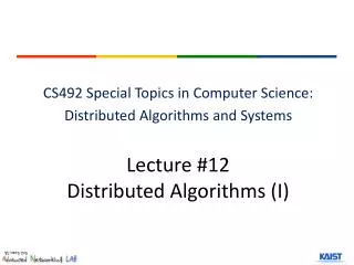
10. P1 P2 r12 r21 P3 r31 r13 r24 P4 r42 SS Algorithm 1:Breadth-first spanning tree • Shared-memory model • Connected, undirected graph G = (V,E), where V = { 1,2,…,n }. • Processes P1,…,Pn, whereP1 is a designated root process. • Some knowledge is permanent: • P1 always knows it’s the root. • Everyone always knows who their neighbors are. • Neighboring processes in G share registers in both directions: • rij written by Pi, read by Pj. • Output: A breadth-first spanning tree, recorded in the rijs as follows: • rij.parent = 1 if j is i’s parent, 0 otherwise. • rij.dist = distance from root to i in the BFS tree = smallest number of hops on any path from 1 to i in G. • Moreover, the values in the registers should remain constant from some point onward.

11. Breadth-first spanning tree • In terms of legal sets: • Define an execution fragment  to be legal if the registers have correct BFS output values, in all states in . • Moreover, registers never change. • L = set of legal execution fragments. • Safe state s: • Global state from which all extensions have registers with correct, unchanging BFS output values. • SS definition says: • Any fair execution fragment , starting from any state, contains some “safe” state s. • That is, one from which all extensions have registers with correct, unchanging BFS output values. • Implies that any fair execution fragment  has a suffix in which the register contents represent a fixed BFS tree.

12. Algorithm strategy • The system can start in any state, with • Any values (of the allowed types) in registers, • Any values in local process variables, • So, the processes can’t assume that their own states and output registers are initially correct. • Recalculate their states and outputs based on inputs from neighbors. • Recalculate at every step: • If recalculate only finite number of times, the initial state could be chosen after the recalculations are finished.

13. You’re not my parent My distance from root Root process P1 do forever for every neighbor m do write r1m := (0,0) • Keep writing (0,0) everywhere. • Access registers in fixed, round-robin order.

14. Non-root process Pi • Maintains local variables lrji to hold latest observed values of incoming registers rji. • First loop: • Read all the rji, copy them intolrji. • Use this local info to calculate new best distance dist, choose a parent that yields this distance. • Use default rule, e.g., smallest index, so always break ties the same way. • Needed for stabilization to a fixed tree. • Second loop: • Write dist to all outgoing registers. • Notify new parent.

15. Non-root process Pi • do forever • for every neighbor m do • lrmi := read(rmi) • dist := min({ lrmi.dist}) + 1 • found := false • for every neighbor m do • if not found and dist = lrmi.dist + 1 then • write rim := (1,dist) • found := true • else • write rim := (0,dist) • Note: • Pi doesn’t take min of its own dist and neighbors’ dists. • Unlike non-SS relaxation algorithms. • Ignores its own dist, recalculates solely from neighbors’ dists. • Because its own value could be erroneous.

16. Correctness • Prove this stabilizes to a particular “default” BFS tree. • Define the default tree to be the unique BFS tree where ties in choosing parent are resolved using rule: • Smallest index yielding the shortest distance. • Prove that, from any starting global state, the algorithm eventually reaches and retains the default BFS tree. • More precisely, show it reaches a safe state, from which any execution fragment retains the default BFS tree. • Show this happens within bounded time: O(diam  l), where • diam is diameter of G (max distance from P1 to anyone is enough). •  is maximum node degree • l is upper bound on local step time • Big-O is about 4.

17. Correctness • Uses a lemma marking progress through distances 0, 1, 2,..., diam, as for basic AsynchBFS. • New complication: Erroneous, too-small distance estimates. • Define a floating distance in a global state to be a value of some rij.dist that is strictly less than the actual distance from P1 to Pi. • Can’t be correct. • Lemma: For every k  0, within time (4k+1)l, we reach a configuration such that: 1. For any i with dist(P1,Pi)  k, every rij.dist is correct. 2. There is no floating distance < k. • Moreover, these properties persist after this configuration.

18. Proof of lemma • Lemma: For every k  0, within time (4k+1)l, we reach a configuration such that: 1. For any i with dist(P1,Pi)  k, every rij.dist is correct. 2. There is no floating distance < k. • Proof: Induction on k. • k = 0: P1 writes (0,0) everywhere within timel. • Assume for k, prove for k+1: • Property 1: • Consider Pi at distance k+1 from P1. • In one more interval of length 4l, Pi has a chance to update its local dist and outgoing register values. • By inductive hypothesis, these updates are based entirely on: • Correct distance values from nodes with distance  k from P1, and • Possibly some floating values, but these must be  k. • So Pi will calculate a correct distance value. • Property 2: • For anyone to calculate a floating distance < k+1, it must see a floating distance < k. • Can’t, by inductive hypothesis.

19. Proof, cont’d • We have proved: • Lemma: For every k  0, within time (4k+1)l, we reach a configuration such that: 1. For any i with dist(P1,Pi)  k, every rij.dist is correct. 2. There is no floating distance < k. • So within time (4 diam +1) l, all the rij.dist values become correct. • Persistence is easy to show. • Once all the rij.dist values are correct, everyone will use the default rule and always obtain the default BFS tree. • Ongoing failures: • If arbitrary failures occur from time to time, not too frequently, the algorithm gravitates back to correct behavior in between failures. • Recovery time depends on size (diameter) of the network.

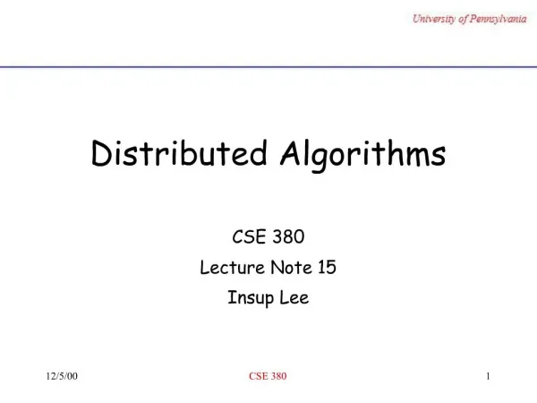
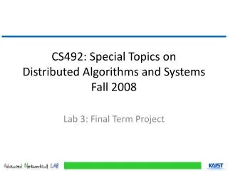
20. x1 xn P1 x2 Pn P2 P3 x3 That’s (n+1), not n. Self-stabilizing mutual exclusion • [Dijkstra 73] • Ring of processes, each with output variable xi. • High granularity: In one atomic step, process Pi can read both neighbors’ variables, compute its next value, and write it to variable xi. P1: do forever: if x1 = xn then x1 := x1 + 1 mod (n+1) Pi, i  1: do forever: if xi xi-1 then xi := xi-1 • That is: • P1 tries to make its variable unequal to its predecessor’s. • Each other tries to make its variable equal to its predecessor’s

21. Mutual exclusion • In what sense does this “solve mutual exclusion”? • Definition: “Pi is enabled” (or “Pi can change its state”) in a configuration, if the variables are set so Pi can take a step and change the value of its variable xi. • Legal execution fragment : • In any state in , exactly one process is enabled. • For each i,  contains infinitely many states in which Pi is enabled. • Use this to solve mutual exclusion: • Say Pi interacts with requesting user Ui. • Pi grants Ui the critical section when: • Ui has requested it, and • Pi is enabled. • When Ui returns the resource, Pi actually does its step, changing xi. • Guarantees mutual exclusion, progress. • Also lockout-freedom.

22. Lemma 1 • Legal : • In any state in , exactly one process is enabled. • For each i,  contains infinitely many states in which Pi is enabled. • Lemma 1: A configuration in which all the x variables have the same value is safe. • Meaning from such a config, any fair execution fragment is legal. • Proof: Only P1 can change its state, then P2,…and so on around the ring (forever). • Remains to show: Starting from any state, we actually reach a configuration in which all the x values are the same.

23. Lemma 2 • Lemma 2: In every configuration, at least one of the potential x values, {0,…,n}, does not appear in any xi. • Proof: Obviously. There are are only n variables and n+1 values.

24. Lemma 3 • Lemma 3: In any fair execution fragment (from any configuration c), P1 changes x1 at least once every nl time. • Proof: • Assume not---P1 goes longer than nl without changing x1 from some value v. • Then by time l, P2 sets x2 to v, • By time 2l, P3 sets x3 to v, • … • By (n-1)l, Pn sets xn to v. • All these values remain = v, as long as x1 doesn’t change. • But then by time nl, P1 sees nl = x1, and changes x1.

25. Lemma 4 • Lemma 4: In any fair execution fragment , a configuration in which all the x values are the same (and so, a safe configuration) occurs within time (n2 + n)l. • Proof: • Let c = initial configuration of . • Let v = some value that doesn’t appear in any xi, in c. • Then v doesn’t appear anywhere, in , unless/until P1 sets x1 := v. • Within time nl, P1 increments x1 (by 1, mod (n+1)). • Within another nl, P1 increments x1 again. • … • Within n2l, P1 increments x1 to v. • Still no other v’s anywhere else… • Then this v propagates all the way around the ring. • P1 doesn’t change x1 until v reaches xn. • Yields all the xi = v, within time (n2 + n)l.

26. Putting the pieces together • Legal execution fragment : • In any state in , exactly one process is enabled. • For each i,  contains infinitely many states in which Pi is enabled. • L = set of legal fragments. • Theorem: Dijkstra’s algorithm is self-stabilizing with respect to legal set L. • Remark: • This uses n+1 values for the xi variables. • Also works with n values, or even n-1. • But not with n-2 [Dolev, p. 20].

27. x1 xn P1 x2 Pn P2 P3 x3 Reducing the atomicity • Dijkstra’s algorithm requires atomic read of xi-1 and write of xi. • Adapt for usual model, in which only individual read/write steps are atomic: • Consider Dijkstra’s algorithm on a 2n-process ring, with processes Qj, vars yj. j = 1, 2, …, 2n. • Needs 2n+1 values for the variables. • Run this in an n-process ring, with processes Pi, variables xi. • Pi emulates both Q2i-1 and Q2i. • y2i-1 is a local variable of Pi. • y2i corresponds to xi. • When Pi emulates a step of Q2i-1, it reads from xi-1, writes to its local variable y2i-1. • When Pi emulates a step of Q2i, it reads from its local variable y2i-1, writes to xi. • Since in each case one variable is internal, can emulate these steps with just read or write.

28. Composing self-stabilizing algorithms • Consider several algorithms, where • A1 is self-stabilizing for legal set L1, • A2 is SS for legal set L2, “assuming A1 stabilizes for L1” • A3 is SS for legal set L3, “assuming A1 stabilizes for L1 and A2 stabilizes for L2” • etc. • Then we should be able to run all the algorithms together, and the combination should be self-stabilizing for L1  L2  L3  … • Need composition theorems. • Details depend on which model we consider. • E.g., consider two shared memory algorithms, A1 and A2.

29. Composing SS algorithms • Consider read/write shared memory algorithms, A1 and A2, where: • A1 has no “unbound” input registers: • All its registers are written, and read, by A1 processes. • A2 has shared registers for its own private use, plus some input registers that are outputs of A1: • Written (possibly read) by processes of A1, only read by processes ofA2. • A1 makes sense in isolation, A2 depends on A1 for some inputs. • Definition: A2 is self-stabilizing (for L2) with respect toA1 (and L1) provided that: If  is any fair execution fragment of the combination of A1 and A2 whose projection onA1 is in L1, then  has a suffix in L2. • Theorem: If A1 is SS for L1 and A2 is SS for L2 with respect toA1 and L1, then the combination of A1 and A2 is SS forL2.

30. Weaker definition of SS • At this point, [Dolev] seems to be using the weaker definition for self-stabilization: • Instead of: • Algorithm A is self-stabilizing for legal set L if every fair execution fragment  of A contains a state s that is safe with respect to L. • Now using: • Algorithm A is self-stabilizing for legal set L if every fair execution fragment  has a suffix in L. • So we’ll switch here.

31. Composing SS algorithms • Def: A2 is self-stabilizing (for L2) with respect toA1 (and L1) provided that any fair execution fragment of the combination of A1 and A2 whose projection onA1 is in L1, has a suffix in L2. • Theorem: If A1 is SS for L1 and A2 is SS for L2 with respect toA1 and L1, then the combination of A1 and A2 is SS forL2. • Proof: • Let  be any fair exec fragment of the combination of A1 and A2 . • We must show that  has a suffix in L2 (weaker definition of SS). • Projection of  on A1 is a fair execution fragment of A1. • Since A1 is SS for L1, this projection has a suffix in L1. • Therefore,  has a suffix  whose projection on A1 is inL1. • Since A2 is self-stabilizing with respect toA1,  has a suffix  in L2. • So  has a suffix in L2, as needed. • Total stabilization time is the sum of the stabilization times of A1 and A2.

32. P1 P2 P3 P4 P5 Applying the composition theorem • Supports modular construction of SS algorithms. • Example: SS mutual exclusion in an arbitrary rooted undirected graph • A1: • Constructs rooted spanning tree, using the SS BFS algorithm. • The rij registers contain all the tree info (parent and distance). • A2: • Takes A1’s rij registers as input. • Solves mutual exclusion using a Dijkstra-like algorithm, which runs on the stable tree in the rij registers. • Q: But Dijkstra’s algorithm uses a ring---how to run it on a tree? • A: Thread the ring through the nodes of the tree, e.g.:

33. P1 P2 P3 P4 P5 Mutual exclusion in a rooted tree • Use the read/write version of the Dijkstra ring algorithm, with local and shared variables. • Each process Pi emulates several processes of Dijkstra algorithm. • Bookkeeping needed, see [Dolev, p. 24-27]. • Initially, both the tree and the mutex algorithm behave badly. • After a while (O(diam  l) time), the tree stabilizes (since the BFS algorithm is SS), but the mutex algorithm continues to behave badly. • After another while (O(n2 l) time), the mutex algorithm also stabilizes (since it’s SS given that the tree is stable). • Total time is the sum of the stabilization times of the two algorithms: O(diam  l) + O( n2 l) = O( n2 l).

34. Self-stabilizing emulations[Dolev, Chapter 4] • Design a SS algorithm A2 to solve a problem L2, using a model that is more powerful then the “real” one. • Design an algorithm A1 using the real model, that “stabilizes to emulate” the powerful model • Combine A1 and A2 to get a SS algorithm for L2 using the real model. • Example [Dolev, Section 4.1]: Scheduling daemon • Rooted undirected graph of processes. • Powerful model: Process can read several variables, change state, write several variables, all atomically. • Real model: just read/write steps. • Emulation algorithm A1: • Uses Dijkstra-style mutex algorithm over BFS spanning tree algorithm • Process performs steps of A2 only when it has the critical section (global lock). • Performs all steps that are performed atomically in the powerful model, before exiting the critical section. • Initially, both emulation A1 and algorithm A2 behave badly. • After a while, emulation begins behaving correctly, yielding mutual exclusion. • After another while, A2 stabilizes for L2.

35. Self-stabilizing emulations • Example 2 [Nolte]: Virtual Node layer for mobile networks • Mobile ad hoc network: Collection of processes running on mobile nodes, communicating via local broadcast. • Powerful model: Also includes stationary Virtual Nodes at fixed geographical locations (e.g., grid points). • Real model: Just the mobile nodes. • Emulation algorithm A1: • Mobile nodes in the vicinity of a Virtual Node’s location cooperate to emulate the VN. • Uses Replicated State Machine strategy, coordinated by a leader. • Application algorithm A2 running over the VN layer: • Geocast, or point-to-point routing, or motion coordination,… • Initially, both the emulation A1and the application algorithm A2 behave badly. • Then the emulation begins behaving correctly, yielding a VN Layer. • Then the application stabilizes.

36. Making non-self-stabilizing algorithms self-stabilizing • [Dolev, Section 2.8]: Recomputation of floating outputs. • Method of converting certain non-SS distributed algorithm to SS algorithms. • What kind of algorithms? • Algorithm A, computes a distributed function based on distributed inputs. • Assumes processes’ inputs are in special, individual input variables, Ii, whose values never change (e.g., contain fixed information about local network topology). • Outputs placed in special, individual output variables Oi. • Main idea: Execute A repeatedly, from its initial state, with the fixed inputs, with two kinds of output variables: • Temporary output variables oi. • Floating output variables FOi. • Use the temporary variables oi the same way A uses Oi. • Write to the floating variables FOi only at the end of function computation. • When restarting A, reset all variables except the floating outputs FOi. • Eventually, the floating outputs should stop changing.

37. Example: Consensus • Consider synchronous, non-fault-tolerant network consensus algorithm. • Undirected graph G = (V,E), known upper bound D on diameter. • Non-SS consensus algorithm A: • Everyone starts with Boolean input in Ii. • After D rounds, everyone agrees, and decision value = 1 iff some input = 1. • At intermediate rounds, process i keeps current consensus proposal in Oi. • At each round, send Oi to neighbors, resets Oi to “or” of its current value and received values. • Stop after D rounds. • A works fine, in synchronous model, if it executes once, from initial states.

38. Example: Consensus • To make this self-stabilizing: • Run algorithm A repeatedly, with the FOi as floating outputs. • While running A, use oi instead of Oi. • Copy oi to FOi at the end of each execution of A. • This is not quite right… • Assumes round numbers are synchronized. • Algorithm begins in an arbitrary global state, round numbers can be off. • So, must also synchronize round numbers 1,2,…,D. • Needs a little subprotocol. • Each process, at each round, sets its round number to max of its own and all those of its neighbors. • When reach D, start over at 1. • Eventually, the rounds become synchronized throughout the network. • Thereafter, the next full execution of A succeeds, produces correct outputs in the FOi variables. • Thereafter, the FOi will never change.

39. Extensions • Can make this into a fairly general transformation, for synchronous algorithms. • Using synchronizers, can extend to some asynchronous algorithms.

40. Making non-SS algorithms SS: Monitoring and resetting • [Section 5.2] • Also known as checking and correction. • Assumes message-passing model. • Basic idea: • Continually monitor the consistency of the underlying algorithm. • Repair the algorithm when inconsistency is detected. • For example: • Use SS leader election service to choose a leader (if there isn’t already a distinguished process). • Leader, repeatedly: • Conducts global snapshots, • Checks consistency, • Sends out corrections if necessary. • Local monitoring and resetting: • For some algorithms, can check and restore local consistency predicates. • E.g., BFS: Can check that local distance is one more than parent’s distance, recalculate dist and parent if not. • [Varghese thesis]

41. Other stuff in the book • Proof methods for showing SS. • Stabilizing to an abstract specification. • Practical motivations. • Model conversions, for SS algorithms: • Shared memory  message-passing • Synchronous  asynchronous • Converting non-SS algorithms to SS algorithms • SS in presence of ongoing failures. • Stopping, Byzantine, message loss. • Efficient “local” SS algorithms. • And many more examples.

42. Next time… • Partially synchronous distributed algorithms • Reading: • Chapters 23-25 • [Dwork, Lynch, Stockmeyer]