Instructions
Instructions. Read the slide notes (under each slide) Review the slide for the main messages Answer questions (correct answers at end) Some advanced/optional slides also at end After completing a slide… …means optionally proceed to SC.63-SC.65 I f unsure: james.brown@hydrosolved.com.


Instructions
E N D
Presentation Transcript
Instructions • Read the slide notes (under each slide) • Review the slide for the main messages • Answer questions (correct answers at end) • Some advanced/optional slides also at end • After completing a slide… • …means optionally proceed to SC.63-SC.65 • If unsure: james.brown@hydrosolved.com SC.63 - SC.65
1stHEFS workshop, 08/19/2014 Basic Hydrologic Ensemble Theory (for review in Seminar C) James Brown james.brown@hydrosolved.com
Contents • Why use ensemble forecasting? • What are the sources of uncertainty? • How to quantify the input uncertainties? • The ingredients of a probability model • How to quantify the output uncertainties? • How to apply operationally?
What is not covered? • Limited scope • Not a mathematical/statistical primer • Not a literature review of current techniques • Focus on the basic theory of ensemble forecasting • Does not cover theory of hindcasting and verification • Limited detail • Mathematical detail often sacrificed • Not focused on HEFS techniques (addressed later) • For more details, see linked resources (end of slides)
Reasons to assess uncertainty • Single-valued forecasts are misleading • There is an understandable desire for simplicity • Yet, also known that large uncertainties are common • Ignoring them can lead to wrong/impaired decisions • Uncertainties “propagate” (e.g. met > hydro > eco) • Risk-based decision making • Knowledge of uncertainty helps to manage risks • E.g. risk of false warnings tied to flood probability • E.g. risk of excess releases tied to inflow probability
Reasons to assess uncertainty National Research Council, 2006 COMPLETING THE FORECAST Characterizing and communicating Uncertainty for Better Decisions Using Weather and Climate Forecasts Committee on Estimating and Communicating Uncertainty in Weather and Climate Forecasts Board on Atmospheric Sciences and Climate Division on Earth and Life Studies NATIONAL RESEARCH COUNCIL OF THE NATIONAL ACADEMIES THE NATIONAL ACADEMIES PRESS Washington, D.C. www.nap.edu “All prediction is inherently uncertain and effective communication of uncertainty information in weather, seasonal climate, and hydrological forecasts benefits users’ decisions (e.g. AMS, 2002; NRC; 2003b). The chaotic character of the atmosphere, coupled with inevitable inadequacies in observations and computer models, results in forecasts that always contain uncertainties. These uncertainties generally increase with forecast lead time and vary with weather situation and location. Uncertainty is thus a fundamental characteristic of weather, seasonal climate, and hydrological prediction, and no forecast is complete without a description of its uncertainty.” [emphasis added]
Example application • HEFS inputs to NYCDEP Operational Support Tool (OST) • Output: risks to volume objectives (e.g. habitat, flooding) • Output: risks to quality objectives (NYC water supply) Initial conditions (reservoir storage/quality; snowpack) [single-valued] Water models Reservoir Water Quality Model (CEQUAL-W2) Reservoir storages, diversions, releases and spills [ensemble] Forcing forecast [single-valued] OASIS Water System Model Effluent turbidity [ensemble] HEFS streamflow forecast [ensemble] Turbidity forecast [single-valued]
Reasons to not assess uncertainty • In the interests of balance… • Technical details risk knowledge/communication gap • Scope for misunderstanding probabilities… • …for example, may not consider all uncertainties • Large upfront investment (in systems and training) • But justified for operational forecasting • For operations, balance strongly favors ensembles • Reflected in investments (NWS, ECMWF, BoM..) • BUT: training and communication is a long-term effort
Reasons to use ensemble technique • Ensemble Prediction Systems • Highly practical tool to “propagate” uncertainty • Based on running models with multiple scenarios • Scenario is one combination of model settings • Need to include all main settings/uncertainty sources • Advantages • Flexible: just run existing (chain of) models n times • Scalable: allows complex models, parallel processing • Collaborative: widely used in meteorology etc.
History of ensembles in NWS • Focused on long-range • Ensemble Streamflow Prediction (since late 1970s) • Climate ensemble from past weather observations • Various adaptations (e.g. to use CPC outlooks) • Limitations of ESP • Not based on forecasts, so only reproduces the past • Does not use best data for short-/medium-range • Does not account for hydrologic uncertainties/biases • Hydrologic uncertainties/biases can exceed meteo.!
Need for an end-to-end system • HEFS service objectives • HEFS “A Team” defined several requirements: • Span lead times from hours to years, seamlessly • Issue reliable probabilities (capture total uncertainty) • Be consistent in space/time, linkable across domains • Use available meteorological forecasts, correct biases • Provide hindcasts consistent w/ operational forecasts • Support verification of the end-to-end system • These requirements are built into HEFS theory
Question 1: check all that apply • What are the limitations of NWS-ESP? • A. Does not model forcing uncertainty • B. Does not model hydrologic uncertainty • C. Does not model total uncertainty • D. Does not use short/medium-range forecast forcing • E. Is not based on calibrated hydrologic models • F. Does not correct for biases • Answers are at the end.
Main sources of uncertainty • Total uncertainty in hydrologic forecasts • Originates from two main sources: • Meteorological forecast uncertainties • Hydrologic modeling uncertainties • Can be further separated into many detailed sources • How do they contribute? • Absolute and relative contributions vary considerably • Data/model factors: forecast horizon, calibration etc. • Physical factors: climate, location, season etc.
Example: two very different basins • Fort Seward, CA (FTSC1) and Dolores, CO (DOSC1) • Total skill in EnsPost-adjusted GFS streamflow forecasts is similar • Origins are completely different (FTSC1=forcing, DOLC2=flow)
Example: two very different seasons • However, in FTSC1, completely different picture in wet vs. dry season • In wet season (which dominates overall results), mainly MEFP skill • In dry season, skill mainly originates from EnsPost (persistence)
How do sources contribute? • Uncertainty in model output depends on • Magnitude of uncertainty in input sources • Sensitivity of the output variable to uncertain inputs • Uncertainty in outputs increases with both factors • Sensitivity is controlled by the model equations • Simple example (one uncertainty source) • Linear reservoir model, with flow equation: • Q=wS • Outflow = watershed coefficient * Storage
How do sources contribute? Q=1.0S Q Slope = “sensitivity” Output uncertainty (Q) Q=0.25S SC.61 S Width = “magnitude” Input uncertainty (S)
How can we capture all sources? • What about non-hydrologic sources? • Hydrologic outputs often used in additional models • Are those uncertainties being considered? • What about social and economic uncertainties? • What constitutes a “source”? • Where to stop? Can always drill down further • Detailed model may be desirable, but rarely practical • Aggregate detailed sources, capturing total uncertainty • For example: meteorological (S1) + hydrologic (S2)
Question 2: check all that apply • Flow forecast uncertainty depends on: • A. Hydrologic uncertainty • B. Meteorological uncertainty • C. Magnitude of input uncertainties • D. Economic and social uncertainties • E. Basin characteristics • F. Sensitivity of model output to each input • Answers are at the end.
Preliminaries: terminology • Error, bias, association • Error: deviation between predicted and “true” outcome • Bias: a consistent error (in one direction) • Association: strength of relationship (ignoring bias) • Uncertainty • Inability to identify single (“true”) outcome • Equivalently: the inability to identify true error • Randomness/unpredictability introduces uncertainty • Need to model the possible errors (uncertainty)
Error, bias, association Observed Forecast Value Time • Unbiased • Strong association • Small total error • Some bias • Moderate association • Moderate total error • Large bias • Strong association • High total error • Unbiased (but conditionally biased) • Negative association • High total error
Uncertainty: range of values Uncertainty is a relative quantity All three forecasts captured the observation Forecast 1 (climatology) Forecast 2 (issued 2 weeks ago) Forecast 3 (issued yesterday) Observation (what happened) Small uncertainty (i.e. much narrower spread than climatology) Probability (density) Large uncertainty (i.e. spread quite similar to climatology) Average temperature, today (C)
Uncertainty: range can be wrong! Capturing forecast uncertainty doesn’t mean always being right! Flooding forecast 23 times with probability 0.4-0.6 (mean=0.48) “When flooding is forecast with probability 0.48, it should occur 48% of the time.” Actually occurs 36% of time. Sample size plot 1.0 0.9 0.8 0.7 0.6 0.5 0.4 0.3 0.2 0.1 0.0 Observed probability of flood given forecast 50 0 Frequency 0.0 0.2 0.4 0.6 0.8 1.0 Forecast class 0 0.1 0.2 0.3 0.4 0.5 0.6 0.7 0.8 0.9 1.0 Forecast probability of flood
Foundations: random variables • What is a random variable? • A variable with several possible outcomes • Actual outcome is unknown (e.g. until observed) • Event is a subset of outcomes (e.g. flows > flood flow) • Strict rules for assigning probabilities to events • Types of (random) variable • Continuous (e.g. temperature) • Discrete (e.g. occurrence of a flood) • Mainly continuous (e.g. precipitation, streamflow) SC.63-SC.65
Assigning probabilities from data • Empirical approach • Observe several (n) past outcomes, tabulate their relative frequencies, and plot histogram • Useful for understanding climatological probabilities. Indeed, this is used for ESP • But, limited to what happened in the past. Also, sample size dependent / noisy • Thus, data often used to help calibrate a model for the probabilities in future. In other words, we use data in a model Moderate flows are relatively likely Skewed distribution with “long tail” Relative frequency (n=100) 100 200 300 400 500 600 700 SC.66 Flow intervals, CMS
Probability density • PDF • Applies to continuous variables only (e.g. temperature, flow) • For continuous variables, probability is defined over an interval. For exact values, the interval is zero, hence Pr=0 • “Probability density function” (PDF) plots the concentration of probability within a tiny interval (infinitely small) • Probability density must not be confused with probability. For example, densities can exceed 1 Moderate temperatures are relatively more likely Probability density function, fT(t) Probability density a Temperature, T (C)
Cumulative probability • CDF • Cumulative probability is the probability that the random variable takes a value less than or equal to the specified value • Plotted for all possible values as a “cumulative distribution function” or CDF • Cumulative probabilities are always between [0,1] and approach 0 at - and 1 at + • Cumulative probabilities are non-decreasing from left to right Cumulative distribution function, FT(t) FT(a) Cumulative probability a SC.68 - SC.69 Temperature, T (C)
Some common PDFs Normal (e.g. temperature) Lognormal (e.g. streamflow) Probability density Weibull (e.g. precipitation) Gamma (e.g. precipitation) Variable value
The remarkable normal distribution • A common shape • Central Limit Theorem: under certain (common) conditions, a sum of random variables is approximately normal • Sums of random variables are common in nature & engineering • Thus, many variables are approx. normally distributed • Normal is a simple shape with many desirable characteristics… • E.g. A linear combination of normal variables is also normal! Mean, , or “expected value” (also the median and mode) Probability density function, fT(t) Probability density Spread, Temperature, T (C)
Estimating parameters of shapes • Model parameters • Fitted probability distributions have parameters to estimate • Parameters dictate location, width, precise shape etc. • Normal distribution is specified by the mean and spread • Different ways to estimate parameters. For example, using historical sample data (right) • When forecasting a random variable, the future parameters depend on the forecast model Mean or “expected” value of the distribution Probability density function, fT(t) Spread or Probability density Temperature, T (C)
Question 3: check all that apply • The normal distribution is: • A. A skewed probability distribution • B. Completely defined by its mean value • C. Symmetric • D. A distribution with equal mean, median and mode • E. Widely used in probability and statistics • F. Applicable to discrete random variables • Answers are at the end.
Marginal & conditional probability • Marginal probability • Simplest case, involving one random variable • For example, streamflow at one time and location • Can be expressed as a PDF or CDF (see above) • Conditional probability • A probability distribution that is subject to conditions • For example, streamflow given that precipitation > 0 • This is expressed as a (conditional) PDF or CDF • We express these conditions if they are important
Joint probability distribution Two random variables (could be more) Pr(X in δxand Y in δy) fY(y) Contours show joint Relationship, fXY(x,y) δy e.g. Y = NYC temperature δx fX(x) e.g. X= Washington DC temperature
Joint probability distribution Contains marginals and conditionals Slice through distribution at x=40F Contours show joint Relationship, fXY(x,y) fY|X(y|x=40) Temperature in NYC, when DC is 40F Temperature in Washington DC is 40F x=40F
Joint probability distribution • What does it tell us? • Contains information about each variable (marginals) • Contains information about how they are related • Could involve multiple times, locations, variables,… • Why do we need to consider this? • Hydrologic models have inputs that are dependent • For example, temperature, precipitation, evaporation • Can’t have “snow” ensemble member at 40C! • Many different ways to model this dependence SC.70
Linear dependence and correlation • Correlation, • Measures degree of linear (not non-linear!) association between two continuous variables, X & Y • For two joint normally distributed variables, correlation captures their joint relationship • Linear modeling is common in hydrometeorology. Thus, correlation is widely used • If input (X) to a linear regression is normal, output (Y) is normal (N) with mean, +X, and variance (2) equal to variance of residual, • . • . • . • . • . • . • . • . • . • . • . • . • . • . • . • . • . • . • . Y • . • . • . • . Temperature in sub-basin S2, Y (C) • . • . • . • . • . • . • . x=40 • . • . • . • . X • . Temperature in sub-basin S1, X (C)
Data transforms • Data transforms are common • Many reasons for data transforms • For example, to suppress extreme values • Power transforms widely used (e.g. Box-Cox) • Often used to make data more normally distributed • Distribution remapping • More aggressive, non-linear, data transformation • Maps distribution of Q to a standard distribution, Z • Normal Quantile Transform (NQT) is one example…
Normal Quantile Transform (NQT) • Transform data to be marginally normal • Need to back-transform each model prediction to flow space Cumulative distribution function of data, FQ(q) Standard normal cdf, FZ(z)=N(0,1) FQ(qz) Cumulative probability Quantile function maps from probability, FQ(qz), to quantile, zq. Quantile function of N(0,1) qz zq Flow, Q (CMS) Normal quantile of flow, Z
Modeling considerations • When theory meets hydrologic reality • Variables often highly skewed, strongly not normal • Space/time and cross-variable relations are complex • Climate/river processes can change (non-stationarity) • Sub-populations often exist (e.g. amount-dependence) • What is the optimal model complexity? • Keep it simple: what can reasonably be ignored? • Limited historical data implies a simpler model… • …otherwise, there’s a real risk of “curve fitting”
Question 4: check all that apply • The correlation coefficient is: • A. A parameter of the bivariate normal distribution • B. A parameter of the marginal normal pdf • C. Always zero for two independent variables • D. Rarely applicable • E. A measure of linear dependence • F. A measure of non-linear dependence • Answers are at the end.
5. How to quantify the output (i.e. forecast) uncertainty? SC.72
Monte Carlo Simulation • Foundation for ensemble prediction • For any model, g, with inputs {X1,…,Xm} and output, Y: • Draw a random sample, {x1,…,xm}, from input joint PDF • Run the model, y1=g(x1,…,xm), and store the result • Repeat n times (e.g. n=1000) or until PDF of Y is stable • Scales up with model complexity • Makes no assumptions about g: just a “black box” • Thus, works for complex, non-linear, models • As accurate as required (i.e. n), but runtime high! SC.73
Importance of unbiased sampling Each sample must be equally likely! Target distribution Target distribution Unbiased sample Unbiased sample Model: Y=X1 Probability density Probability density Output, Y Input, X1 Target distribution Target distribution Biased sample Biased sample Model: Y=X1 Probability density Probability density Output, Y Input, X1
Simple random sampling • Sampling any CDF • Many different approaches to random sampling, depending on probability distribution • Simplest, generic, approach is “inverse transform sampling” • Start with a standard Uniform distribution, U(0,1) • Any pseudo-random number generator samples from U(0,1) • For random sample, u1,…,un, transform numbers to target distribution, FT(t), as Cumulative distribution function or cdf, FT(t) u1 u2 u3 Cumulative probability t1 t2 t3 Temperature, T (C)
Question 5: check all that apply • Monte Carlo simulation requires: • A. A simple forecast model • B. An equal chance of sampling each possible value • C. The joint probability distribution of model inputs • D. Uncorrelated inputs • E. Running the forecast model many (n) times • F. An infinitely large sample size • Answers are at the end.
6. Applying the theory to operational forecasting in hydrology