Semi-Supervised Learning

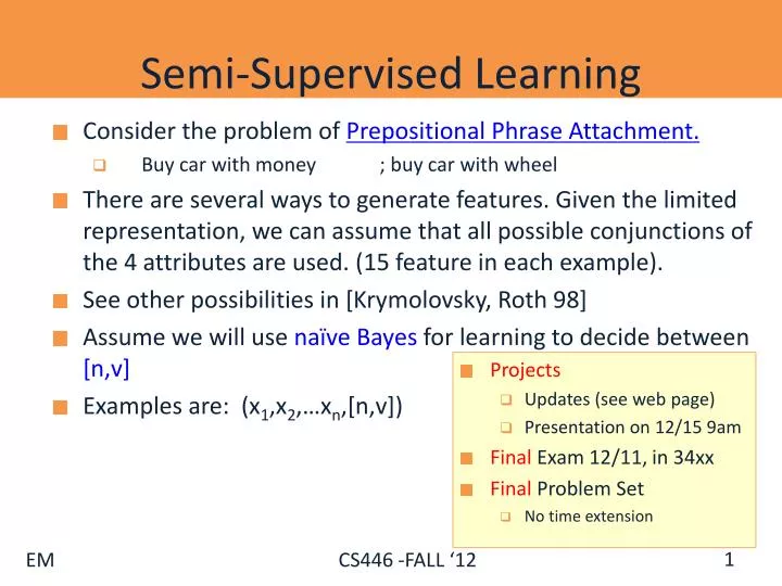
Semi-Supervised Learning • Projects • Updates (see web page) • Presentation on 12/15 9am • FinalExam 12/11, in 34xx • Final Problem Set • No time extension • Consider the problem of Prepositional Phrase Attachment. • Buy car with money ; buy car with wheel • There are several ways to generate features. Given the limited representation, we can assume that all possible conjunctions of the 4 attributes are used. (15 feature in each example). • See other possibilities in [Krymolovsky, Roth 98] • Assume we will use naïve Bayes for learning to decide between [n,v] • Examples are: (x1,x2,…xn,[n,v])

Using naïve Bayes After seeing 10 examples, we have: P(n) =0.5; P(v)=0.5 P(x1|n)=0.75;P(x2|n) =0.5; P(x3|n) =0.5; P(x4|n) =0.5 P(x1|v)=0.25; P(x2|v) =0.25;P(x3|v) =0.75;P(x4|v) =0.5 Then, given an example (1000), we have: Pn(x)~=0.5 0.75 0.5 0.5 0.5 = 3/64 Pv(x)~=0.5 0.25 0.75 0.25 0.5=3/256 Now, assume that in addition to the 10 labeled examples, we also have 100 unlabeled examples.

Using naïve Bayes • For example, what can be done with (1000?) ? • We can guess the label of the unlabeled example… • But, can we use it to improve the classifier (that is, the estimation of the probabilities that we will use in the future)? • We can make predictions, and believe them • Or some of them (based on what?) • We can assume the example x=(1000) is a • An n-labeled example with probability Pn(x)/(Pn(x) + Pv(x)) • A v-labeled example with probability Pv(x)/(Pn(x) + Pv(x)) • Estimation of probabilities does not require working with integers!

Using Unlabeled Data The discussion suggests several algorithms: • Use a threshold. Chose examples labeled with high confidence. Labeled them [n,v]. Retrain. • Use fractional examples. Label the examples with fractional labels [p of n, (1-p) of v]. Retrain.

Comments on Unlabeled Data Both algorithms suggested can be used iteratively. Both algorithms can be used with other classifiers, not only naïve Bayes. The only requirement – a robust confidence measure in the classification. E.g.: Brill, ACL’01: uses all three algorithms in SNoW for studies of these sort. There are other approaches to Semi-Supervised learning: See included papers (co-training; Yarowksy’s Decision List/Bootstrapping algorithm) What happens if instead of 10 labeled examples we start with 0 labeled examples? Make a Guess; continue as above; a version of EM

EM EM is a class of algorithms that is used to estimate a probability distribution in the presence of missing attributes. Using it, requires an assumption on the underlying probability distribution. The algorithm can be very sensitive to this assumption and to the starting point (that is, the initial guess of parameters. In general, known to converge to a local maximum of the maximum likelihood function.

Three Coin Example • We observe a series of coin tosses generated in the following way: • A person has three coins. • Coin 0: probability of Head is  • Coin 1: probability of Head p • Coin 2: probability of Head q • Consider the following coin-tossing scenarios:

Estimation Problems Coin 0 There is no known analytical solution to this problem(general setting). That is, it is not known how to compute the values of the parameters so as to maximize the likelihood of the data. nth toss 2nd toss 1st toss Scenario I: Toss one of the coins six times. Observing HHHTHT Question: Which coin is more likely to produce this sequence ? Scenario II: Toss coin 0. If Head – toss coin 1; o/w – toss coin 2 Observing the sequence HHHHT, THTHT, HHHHT, HHTTH produced by Coin 0 , Coin1 and Coin2 Question: Estimate most likely values for p, q (the probability of H in each coin) and the probability to use each of the coins () Scenario III: Toss coin 0. If Head – toss coin 1; o/w – toss coin 2 Observing the sequence HHHT, HTHT, HHHT, HTTH produced by Coin 1 and/or Coin 2 Question: Estimate most likely values for p, q and 

Key Intuition (1) If we knew which of the data points (HHHT), (HTHT), (HTTH) came from Coin1 and which from Coin2, there was no problem. Recall that the “simple” estimation is the ML estimation: Assume that you toss a (p,1-p) coin m times and get k Heads m-k Tails. log[P(D|p)] = log [ pk (1-p)m-k ]= k log p + (m-k) log (1-p) To maximize, set the derivative w.r.t. p equal to 0: d log P(D|p)/dp = k/p – (m-k)/(1-p) = 0 Solving this for p, gives: p=k/m

Key Intuition (2) If we knew which of the data points (HHHT), (HTHT), (HTTH) came from Coin1 and which from Coin2, there was no problem. Instead, use an iterative approach for estimating the parameters: Guess the probability that a given data point came from Coin 1 or 2 Generate fictional labels, weighted according to this probability. Now, compute the most likely value of the parameters. [recall NB example] Compute the likelihood of the data given this model. Re-estimate the initial parameter setting: set them to maximize the likelihood of the data. (Labels  Model Parameters) Likelihood of the data This process can be iterated and can be shown to converge to a local maximum of the likelihood function

We will assume (for a minute) that we know the parameters and use it to estimate which Coin it is (Problem 1) Then, we will use this estimation to “label” the observed tosses, and then use these “labels” to estimate the most likely parameters and so on... What is the probability that the ith data point came from Coin1 ? EM Algorithm (Coins) -I

Now, we would like to compute the likelihood of the data, and find the parameters that maximize it. We will maximize the log likelihood of the data (mdata points) LL = imlogP(Di |p,q,) But, one of the variables – the coin’s name - is hidden. We can marginalize: LL= i=1mlog y=0,1 P(Di, y | p,q, ) However, the sum is inside the log, making ML solution difficult. Since the latent variable yis not observed, we cannot use the complete-data log likelihood. Instead, we use the expectation of the complete-data log likelihood under the posterior distribution of the latent variable to approximate log p(Di| p’,q’,®’) We think of the likelihood logP(Di|p’,q’,’) as a random variable that depends on the value y of the coin in the ith toss. Therefore, instead of maximizing the LL we will maximize the expectation of this random variable (over the coin’s name). EM Algorithm (Coins) - II

We maximize the expectation of this random variable (over the coin name). E[LL] = E[i=1mlog P(Di,y| p,q, )] = i=1mE[log P(Di, y | p,q, )] = = i=1mP1i log P(Di, 1 | p,q, )] + (1-P1i) log P(Di, 0 | p,q, )] Due to the linearity of the expectation and the random variable definition: P(Di, y | p,q, ) = log P(Di, 1 | p,q, ) with Probability P1i log P(Di, 0 | p,q, ) with Probability (1-P1i) EM Algorithm (Coins) - III

Explicitly, we get: EM Algorithm (Coins) - IV

Finally, to find the most likely parameters, we maximize the derivatives with respect to : Sanity check: Think of the weighted fictional points When computing the derivatives, notice P1i here is a constant; it was computed using the current parameters (including ®). EM Algorithm (Coins) - V

Models with Hidden Variables

The General EM Procedure E M

EM is a general procedure for learning in the presence of unobserved variables. We have shown how to use it in order to estimate the most likely density function for a mixture of (Bernoulli) distributions. EM is an iterative algorithm that can be shown to converge to a local maximum of the likelihood function. It depends on assuming a family of probability distributions. In this sense, it is a family of algorithms. The update rules you will derive depend on the model assumed. It has been shown to be quite useful in practice, when the assumption made on the probability distribution are correct, but can fail otherwise. EM Summary (so far)

EM is a general procedure for learning in the presence of unobserved variables. The (family of ) probability distribution is known; the problem is to estimate its parameters In the presence of hidden variables, we can typically think about it as a problem of a mixture of distributions – the participating distributions are known, we need to estimate: Parameters of the distributions The mixture policy Our previous example: Mixture of Bernoulli distributions EM Summary (so far)

Example: K-Means Algorithm K- means is a clustering algorithm. We are given data points, known to be sampled independently from a mixture of k Normal distributions, with means i, i=1,…k and the same standard variation 

Example: K-Means Algorithm First, notice that if we knew that all the data points are taken from a normal distribution with mean  , finding its most likely value is easy. We get many data points, D = {x1,…,xm} Maximizing the log-likelihood is equivalent to minimizing: Calculate the derivative with respect to , we get that the minimal point, that is, the most likely mean is

A mixture of Distributions As in the coin example, the problem is that data is sampled from a mixture of k different normal distributions, and we do not know, for a given data point xi, where is it sampled from. Assume that we observe data point xi ;what is the probability that was sampled from the distribution j ?

A Mixture of Distributions As in the coin example, the problem is that data is sampled from a mixture of k different normal distributions, and we do not know, for a given each data point xi, where is it sampled from. For a data point xi, define k binary hidden variables, zi1,zi2,…,zik, s.t zij =1iffxi is sampled from the j-th distribution.

The EM Algorithm • Algorithm: • Guess initial values for the hypothesis h= • Expectation: Calculate Q(h’,h) = E(Log P(Y|h’) | h, X) • using the current hypothesis h and the observed data X. • Maximization: Replace the current hypothesis h by h’, that maximizes the Q function (the likelihood function) • set h = h’, such that Q(h’,h) is maximal • Repeat: Estimate the Expectation again.

Example: K-Means Algorithms Expectation: Computing the likelihood given the observed data D = {x1,…,xm} and the hypothesis h (w/o the constant coefficient)

Example: K-Means Algorithms Maximization: Maximizing with respect to we get that: Which yields:

Summary: K-Means Algorithms Given a set D = {x1,…,xm} of data points, guess initial parameters Compute (for all i,j) and a new set of means: repeat to convergence Notice that this algorithm will find the best k points in the sense of minimizing the sum of square distance.

Summary: EM • EM is a general procedure for learning in the presence of unobservable variables. • We have shown how to use it in order to estimate the most likely density function for a mixture of probability distributions. • EM is an iterative algorithm that can be shown to converge to a local maximum of the likelihood function. • It depends on assuming a family of probability distributions. • It has been shown to be quite useful in practice, when the assumption made on the probability distribution are correct, but can fail otherwise. • As examples, we have derived an important clustering algorithm, the k-means algorithm and have shown how to use it in order to estimate the most likely density function for a mixture of probability distributions.

More Thoughts about EM • Assume that a set xi2 {0,1}n+1 of data points is generated as follows: • Postulate a hidden variable Z, with k values, 1 · z · k with probability ®z, 1,k®z = 1 • Having randomly chosen a value z for the hidden variable, we choose the value xi for each observable Xi to be 1 with probability piz and 0 otherwise. • Training: a sample of data points, (x0, x1 ,…, xn) 2 {0,1}n+1 • Task: predict the value of x0, given assignments to all n variables.

More Thoughts about EM • Two options: • Parametric: estimate the model using EM. Once a model is known, use it to make predictions. • Problem: Cannot use EM directly without an additional assumption on the way data is generated. • Non-Parametric: Learn x0 directly as a function of the other variables. • Problem: which function to try and learn? • It turns out to be a linear function of the other variables, when k=2 (what does it mean)? • When k is known, the EM approach performs well; if an incorrect value is assumed the estimation fail; the linear methods performs better [Grove & Roth 2001]

Semi-Supervised Learning