Download

1 / 60
600 likes | 798 Views
PCA and Hebb Rule 0368-4149-01. Prof. Nathan Intrator Tuesday 16:00-19:00 Office hours: Wed 4-5 nin@tau.ac.il cs.tau.ac.il/~nin. Outline . Goals for neural learning - Unsupervised Goals for statistical/computational learning PCA ICA Exploratory Projection Pursuit

E N D
PCA and Hebb Rule0368-4149-01 Prof. Nathan Intrator Tuesday 16:00-19:00 Office hours: Wed 4-5 nin@tau.ac.il cs.tau.ac.il/~nin
Outline • Goals for neural learning - Unsupervised • Goals for statistical/computational learning • PCA • ICA • Exploratory Projection Pursuit • Search for non-Gaussian distributions • Practical implementations
Statistical Approach to Unsupervised Learning • Understanding the nature of data variability • Modeling the data (sometimes very flexible model) • Understanding the nature of the noise • Applying prior knowledge • Extracting features based on: • Prior knowledge • Class prediction • Unsupervised learning
n-dimensional vectors m-dimensional vectors m < n Ex: Neuronal Goal We look for axes which minimise projection errors and maximise the variance after projection transform from 2 to 1 dimension
more information (variance) rotate less information project Algorithm (cont’d) • Preserve as much of the variance as possible
Linear transformations – example 2D vectors X in a unit circle with mean (1,1); Y = A*X, A = 2x2 matrix The shape is elongated, rotated and the mean is shifted.
Invariant distances Euclidean distance is not invariant to general linear transformations This is invariant only for orthonormal matrices ATA = I that make rigid rotations, without stretching or shrinking distances. Idea: standardize the data in some way to create invariant distances.
Data standardization For each vector component X(j)T=(X1(j), ... Xd(j)),j=1 .. n calculate mean and std: n– number of vectors, d – their dimension Vector of mean feature values. Averages over rows.
Standard deviation Calculate standard deviation: Vector of mean feature values. Variance = square of standard deviation (std), sum of all deviations from the mean value. Transform X => Z, standardized data vectors
Std data Std data: zero mean and unit variance. Standardize data after making data transformation. Effect: data is invariant to scaling only (diagonal transformation). Distances are invariant, data distribution is the same?? How to make data invariant to any linear transformations?
Terminology (Covariance) • How two dimensions vary from the mean with respect to each other • cov(X,Y)>0: Dimensions increase together • cov(X,Y)<0: One increases, one decreases • cov(X,Y)=0: Dimensions are independent
Terminology (Covariance Matrix) • Contains covariance values between all possible dimensions: • Example for three dimensions (x,y,z) (Always symetric): cov(x,x) variance of component x
Properties of the Cov matrix • Can be used for creating a distance that is not sensitive to linear transformation • Can be used to find directions which maximize the variance • Determines a Gaussian distribution uniquely (up to a shift)
Data standardization example Transformation Vector of mean feature values. Variance check it! For our example Y=AX, assuming X means=1 and variances = 1 How to make this invariant?
Covariance matrix Variance (spread around mean value) + correlation between features. CXisd x d where X is d x n dimensional matrix of vectors shifted to their means. Covariance matrix is symmetric Cij = Cjiand positive definite. Diagonal elements are variances (square of std), si2 = Cii Pearson correlation coefficient Spherical distribution of data has Cij=I (unit matrix). Elongated ellipsoids: large off-diagonal elements, strong correlations between features.
Mahalanobis distance Linear combinations of features leads to rotations and scaling of data. Mahalanobis distance: is invariant to linear transformations:
Principal components How to avoid correlated features? Correlations covariance matrix is non-diagonal ! Solution: diagonalize it, then use transformation that makes it diagonal to de-correlate features. Z are the eigen vectors of Cx In matrix form, X, Y are dxn, Z, CX,CY are dxd C – symmetric, positive definite matrix XTCX > 0 for ||X||>0; its eigenvectors are orthonormal: its eigenvalues are all non-negative Z – matrix of orthonormal eigenvectors (because Z is real+symmetric), transforms X into Y, with diagonal CY, i.e. decorrelated.
Matrix form Eigenproblem for C matrix in matrix form:
Principal components Z – principal components, of vectors X transformed using eigenvectors of CX Covariance matrix of transformed vectors is diagonal => ellipsoidal distribution of data. PCA: old idea, C. Pearson (1901), H. Hotelling 1933 Result: PC are linear combinations of all features, providing new uncorrelated features, with diagonal covariance matrix = eigenvalues. Small li small variance data change little in direction Yi PCA minimizes C matrix reconstruction errors: Zivectors for large li are sufficient to get: because vectors for small eigenvalues will have very small contribution to the covariance matrix.
Two components for visualization Diagonalization methods: see Numerical Recipes, www.nr.com New coordinate system: axis ordered according to variance = size of the eigenvalue. First k dimensions account for fraction of all variance (please note that li are variances); frequently 80-90% is sufficient for rough description.
Solving for Eigenvalues & Eigenvectors • Vectors x having same direction as Ax are called eigenvectors of A (A is an n by n matrix). • In the equation Ax=x, is called an eigenvalue of A. • Ax=x (A-I)x=0 • How to calculate x and : • Calculate det(A-I), yields a polynomial (degree n) • Determine roots to det(A-I)=0, roots are eigenvalues • Solve (A- I) x=0 for each to obtain eigenvectors x
PCA properties PC Analysis (PCA) may be achieved by: • transformation making covariance matrix diagonal • projecting the data on a line for which the sums of squares of distances from original points to projections is minimal. • orthogonal transformation to new variables that have stationary variances True covariance matrices are usually not known, estimated from data. This works well on single-cluster data; more complex structure may require local PCA, separately for each cluster. PC is useful for: finding new, more informative, uncorrelated features; reducing dimensionality: reject low variance features, reconstructing covariance matrices from low-dim data.
PCA Wisconsin example Wisconsin Breast Cancer data: • Collected at the University of Wisconsin Hospitals, USA. • 699 cases, 458 (65.5%) benign (red), 241 malignant (green). • 9 features: quantized 1, 2 .. 10, cell properties, ex: Clump Thickness, Uniformity of Cell Size, Shape, Marginal Adhesion, Single Epithelial Cell Size, Bare Nuclei, Bland Chromatin, Normal Nucleoli, Mitoses. 2D scatterograms do not show any structure no matter which subspaces are taken!
Example cont. PC gives useful information already in 2D. Taking first PCA component of the standardized data: If (Y1>0.41) then benign else malignant 18 errors/699 cases = 97.4% Transformed vectors are not standardized, std’s are below. Eigenvalues converge slowly, but classes are separated well.
PCA disadvantages Useful for dimensionality reduction but: • Largest variance determines which components are used, but does not guarantee interesting viewpoint for clustering data. • The meaning of features is lost when linear combinations are formed. Analysis of coefficients in Z1 and other important eigenvectors may show which original features are given much weight. PCA may be also done in an efficient way by performing singular value decomposition of the standardized data matrix. PCA is also called Karhuen-Loève transformation. Many variants of PCA are described in A. Webb, Statistical pattern recognition, J. Wiley 2002, good review in Duda and Hart (1973).
Exercise (part 1, Updated Mar 10) • How would you calculate efficiently the PCA of data where the dimensionality d is much larger than the number of vector observations n? • Download the Wisconsin Data from the UC Irvine repository, extract PCAs from the data, test scatter plots of original data and after projecting onto the principal components, plot Eigen values
Unsupervised learning • The Hebb rule – Neurons that fire together wire together. • PCA • RF development with PCA
Classical Conditioning and Hebb’s rule Ear A Nose B Tongue “When an axon in cell A is near enough to excite cell B and repeatedly and persistently takes part in firing it, some growth process or metabolic change takes place in one or both cells such that A’s efficacy in firing B is increased” D. O. Hebb (1949)
The generalized Hebb rule: where xiare the inputs and y the output is assumed linear: Results in 2D
Example of Hebb in 2D w (Note: here inputs have a mean of zero)
In the simplest case, the change in synaptic weight w is: where x are input vectors and y is the neural response. Assume for simplicity a linear neuron: So we get: Now take an average with respect to the distribution of inputs, get:
If a small change Δw occurs over a short time Δt then: (in matrix notation) If <x>=0 , Q is the covariance function. What is then the solution of this simple first order linear ODE ? (Show on board)
Mathematics of the generalized Hebb rule The change in synaptic weight w is: where x are input vectors and y is the neural response: Assume for simplicity a linear neuron: So we get:
Taking an average of the distribution of inputs And using and We obtain
In matrix form Where J is a matrix of ones, e is a vector in direction (1,1,1 … 1), and or Where
The equation therefore has the form If k1 is not zero, this has a fixed point, however it is usually not stable. If k1=0 then have:
The Hebb rule is unstable – how can it be stabilized while preserving its properties? The stabilized Hebb (Oja) rule. Where: Appoximateto first order in η: Now insert Get: Normalize
} y Therefore The Oja rule therefore has the form:
Average In matrix form:
Using this rule the weight vector converges to • the eigen-vector of Q with the highest eigen-value. It is often called a principal component or PCA rule. • The exact dynamics of the Oja rule have been solved by Wyatt and Elfaldel 1995 • Variants of networks that extract several principal components have been proposed (e.g: Sanger 1989)
2 skewed distributions PCA transformation for 2D data: First component will be chosen along the largest variance line, both clusters will strongly overlap, no interesting structure will be visible. In fact projection to orthogonal axis to the first PCA component has much more discriminating power. Discriminant coordinates should be used to reveal class structure.
PCA and FDA are linear, PP may be linear or non-linear. Find interesting “criterion of fit”, or “figure of merit” function, that allows for low-dim (usually 2D or 3D) projection. Projection Pursuit (PP) General transformation with parameters W. Index of “interestingness” Interesting indices may use a priori knowledge about the problem: 1. mean nearest neighbor distance – increase clustering of Y(j)2. maximize mutual information between classes and features 3. find projection that have non-Gaussian distributions. The last index does not use a priori knowledge; it leads to the Independent Component Analysis (ICA).ICA features are not only uncorrelated, but also independent.
ICA is a special version of PP, recently very popular. Gaussian distributions of variable Y are characterized by 2 parameters: mean value: variance: These are the first 2 moments of distribution; all higher are 0 for G(Y). Kurtosis One simple measure of non-Gaussianity of projections is the 4-th moment (cumulant) of the distribution, called kurtosis, measures “skewedness” of the distribution. For E{Y}=0 kurtosis is: Super-Gaussian distribution: long tail, peak at zero, k4(y)>0, like binary image data. sub-Gaussian distribution is more flat and has k4(y)<0, like speech signal data.
Features Yi, Yjare uncorrelated if covariance is diagonal, or: Correlation and independence Variables are statistically independent if their joint probability distribution is a product of probabilities for all variables: Uncorrelated features are orthogonal. Statistically independent features Yi, Yj for any functions give: This is much stronger condition than correlation; in particular the functions may be powers of variables; any non-Gaussian distribution after PCA transformation will still have correlated features.
Example: PCA and PP based on maximal kurtosis: note nice separation of the blue class. PP/ICA example
Some remarks • Many formulations of PP and ICA methods exist. • PP is used for data visualization and dimensionality reduction. • Nonlinear projections are frequently considered, but solutions are more numerically intensive. • PCA may also be viewed as PP, max (for standardized data): Index I(Y;W) is based here on maximum variance. Other components are found in the space orthogonal to W1TX Same index is used, with projection on space orthogonal to k-1 PCs.
How do we find multiple Projections • Statistical approach is complicated: • Perform a transformation on the data to eliminate structure in the already found direction • Then perform PP again • Neural Comp approach: Lateral Inhibition
How do we find multiple Projections – Visual Approach High Dimensional Data Dimension Reduction Visualisation Classification Analysis Feature Extraction