Download
1 / 114
1.14k likes | 1.53k Views
Income Comparisons, the Easterlin Paradox and Public Policy. Andrew E. Clark (Paris School of Economics and IZA) http://www.parisschoolofeconomics.com/clark-andrew/. APE/ETE Masters Course.

E N D
Income Comparisons, the Easterlin Paradox and Public Policy Andrew E. Clark (Paris School of Economicsand IZA) http://www.parisschoolofeconomics.com/clark-andrew/ APE/ETE Masters Course
You might think that money might help us to achieve the variety of different kinds of well-being that have been put forward as important in the literature. Being poor certainly prevents us from doing many things that we would like to do. If you don’t believe me, then try it… But in addition to wishful thinking, what does the data say?
One of the first, and most original, researchers in this area is Dick Easterlin (University of Southern California). He has asked two questions: Are richer individuals/countries happier than poorer individuals/countries? As countries get richer, does everyone become happier? We might expect the answer to these two questions to be the same.
I here present some of the results from: Easterlin, R. A. (2005). “Diminishing Marginal Utility of Income? Caveat Emptor”. Social Indicators Research. pp. 243-255. This specifically deals with the case of Japan. Japan was a poor country in the 1950s/early 1960s, but then experienced unprecedented growth.
Fact 1. Richer countries are happier countries. The blue lines show the estimated relationship between income and happiness Japan Japan was in the middle of the income distribution in the early 1960s, and had a middling level of happiness
So what happened as Japan became richer? Look at annual indices (1962=100) of life satisfaction and real GNP per capita for Japan, 1958-1987 Between 1962 and 1987 Japan experienced unprecedented economic growth, with GNP per capita (in real terms)rising 3.5-fold: growing from 22 to 77 percent of the United States level in 1962 We might then imagine that Japan would follow the blue lines above: as Japan became richer, it would become happier.
In fact, happiness remained constant despite Japan’s remarkable economic growth What “should” have happened What did happen
Are the Japanese strange? Not necessarily: the same thing can be observed in 30 years of American GSS data This is the Easterlin Paradox. Richer individuals are happier, but as countries become richer over time they do not become happier. The challenge to social science is to try to explain why.
This finding has generated a considerable amount of controversy: it just MUST be wrong One point to remember is that the Easterlin Paradox is a statement of why continuous GDP growth may not increase social welfare in the long-run. It is not a theory of recessions not mattering: we shouldn’t be surprised if life satisfaction and the economic cycle are correlated in the short run After all, unemployment is a robust significant indicator of individual subjective well-being (the blips in the US happiness line correspond to the business cycle)
Recent work has considered (and reconsidered) time–series evidence suggesting that the average well-being lines over time above are “really” flat One well-known contribution is Stevenson and Wolfers (2008) There are issues with data comparability over time in Japan: the questions changed over time
Recent work has considered (and reconsidered) time–series evidence suggesting that the average well-being lines over time above are “really” flat SW agree that life satisfaction in the USA follows the business cycle. But also that there is no trend in the GSS data.
Recent work has considered (and reconsidered) time–series evidence suggesting that the average well-being lines over time above are “really” flat There is a positive trend in both happiness and life satisfaction scores in the World Values Survey. Easterlin points out that the trend in WVS happiness scores came from a change in the way the happiness question was administered. And one of the two positive life satisfaction slopes is entirely driven by the recovery of transition countries. While the other relies on two data points (and so wouldn’t survive a jackknife analysis)
United Kingdom (BHPS): Real GDP per capita and life satisfaction 1996 - 2008
West Germany (SOEP): Real GDP per capita and life satisfaction 1984 - 2010
Australia (HILDA): Real GDP per capita and life satisfaction 2001 - 2009
Life Satisfaction in Five European Countries, (World Database of Happiness) 1973-2004
It is easy to lose the will to live when reading the attacks and counter-attacks. There are fundamental issues with the analysis of time-series happiness data.
It is easy to lose the will to live when reading the attacks and counter-attacks. There are fundamental issues with the analysis of time-series happiness data. 1) It is time-series happiness data. So we are making strong statements off of differences in slopes estimated using 20, or 10, or 4 observations.
It is easy to lose the will to live when reading the attacks and counter-attacks. There are fundamental issues with the analysis of time-series happiness data. It is time-series happiness data. So we are making strong statements off of differences in slopes estimated using 20, or 10, or 4 observations. There are never any control variables (age, sex, education, country of birth, urban/rural, labour force status, marital status, and so on): how much of this is a composition effect?
It is time-series happiness data. So we are making strong statements off of differences in slopes estimated using 20, or 10, or 4 observations. There are never any control variables (age, sex, education, country of birth, urban/rural, labour force status, marital status, and so on): how much of this is a composition effect? There are never any macro control variables It is easy to imagine macro “omitted variables” which may obscure the effect of income: inequality, crime, pollution etc.
Perhaps we should stop looking at time series We often appeal to the notion of relative utility, whereby W = W(y, y*, …) to explain the Easterlin Paradox. So let’s turn the question around: if we find strong and consistent evidence of a role of some benchmark or comparison income in individual well-being, then the Easterlin Paradox must at least partly hold: - Then the time-series and cross-section relationships between subjective well-being and income cannot be the same
BROAD IDEA A common idea across the Social Sciences: well-being or utility depends on some kind of comparison process of what you have relative to a reference level. Comparisons can be over “things” or over money. An example. Two people, A and B, who live next to each other, both like cars. WA = W(CarA,.....) WB = W(CarB,.....) Where “W” is the individual’s well-being function.
Key question: is A more likely to buy a new car if B buys a new one? Standard economic theory: No. Comparisons/relative utility: Yes. If the answer is “yes”, then we could write A’s “happiness function” as WA = W(CarA/CarB,....): how good is my car relative to my neighbour’s?
This might sound like a ridiculous proposition. It isn’t, at least not in the Netherlands. Kuhn, P., Kooreman, P., Soetevent, A., and Kapteyn, A. (2011). "The Effects of Lottery Prizes on Winners and their Neighbors: Evidence from the Dutch Postcode Lottery". American Economic Review, 101, 2226-2247. Each week, the Dutch Postcode Lottery (PCL) randomly selects a postal code, and distributes cash and a new BMW to lottery participants in that code.
There are 430 000 postodes in the Netherlands. An average postcode includes around 20 households. A winning participant wins €12,500 per ticket. In addition, one participating household in the winning postcode receives a new BMW. Households in postcodes surveyed six months after the prize was won.
PCL nonparticipants who live next door to winners have significantly higher levels of car consumption than other nonparticipants (sig. levels are all relative to column 2, the non-participants in non-winning PCs)
Applied to Income, instead of Cars: Income and Subjective Well-Being (SWB) Standard model: W = W(y, ....) Comparisons: W = W(y/y*, ....) This is analogous to the car example. The variable y* is “comparison income”: the income to which we compare/income of the reference group.
I mostly consider evidence here resulting from direct measurement of “W”, via job satisfaction, life satisfaction, mental stress etc. Validated by physiological/neurological studies, third-party raters, and (most importantly) future behaviours such as divorce, unemployment duration, quitting one’s job, and morbidity and mortality. There is nothing to stop us looking at behaviours too: I think of the analysis of behaviour and proxy measures of utility as complements, not substitutes.
To whom do we compare? Peer group/people like me Others in the same household Spouse/partner Myself in the past Friends Neighbours Work colleagues “Expectations”
We typically know nothing about the reference group. Wave 3 of the European Social Survey (22 countries) helps here.
Income and comparison intensity are negatively correlated, both within and between countries
Mostly we just impose a reference group, such as people like me, neighbours or family. I use the British Household Panel Study (BHPS) to look at the relationship between job satisfaction and labour income. Main findings: There is some evidence that job satisfaction is an increasing function of income. However, job satisfaction falls as others’ income rises. This holds for: The income of “people like you” (same characteristics, same type of job). Partner’s income. The income of other adults in the same household. The income that you yourself earned in the same job one year ago.
Clark and Oswald (1996). BHPS Data on 5000 Employees Log income (y) -0.02 0.11 -0.001 (0.039) (0.050) (0.04) Log comparison income (y*) --- -0.20 --- (0.062) Log NES comparison income (y**) --- --- -0.26 (0.073) “Comparison Income” predicted from a Mincer Earnings equation (note: requires exclusion restrictions to avoid multicollinearity); “NES comparison income” matched in from another data set by hours of work, and thus avoids identification problems (but assumes reference group defined by hours of work).
Clark (1996). BHPS Data on 5000 Employees Estimated only on couples where both partners are in work. Includes other standard control variables.
Comparisons to the past: Clark (1999). BHPS Data Two waves only. Estimated on individuals who did not change job or get promoted between the two waves.
Therefore, when we look at the effect of own pay and others’ pay on satisfaction, we find the following kind of stylised relationships: Income DOES bring happiness... As long as you get it and no-one else does Satisfaction Own pay (y), holding y* constant
Satisfaction Others’ pay (y*), holding y constant
Satisfaction Pay rises for everybody (y/y* constant) Others have replicated these broad findings with work on life satisfaction and local area average incomes: Ferrer-i-Carbonell for Germany, and Luttmer for the US.
There are three reasons to wonder whether these comparison income results are entirely right: • The Danish • Tunnels • Altruism
From January 1, 2007, Denmark has been split up into five Regions: two in Zealand, two in Jutland, and one covering Funen and Southern Jutland. • Previous to this, Denmark was split up into 15 counties, and 273 municipalities. • We use new geo-referenced data, based on a geographical grid of size 100*100 meters (i.e. 10 000 square meters, or a hectare) covering the entire country.
Some of these grid cells are uninhabited, others are only very thinly inhabited: around two-thirds of inhabited hectare cells contain under five households. • Data confidentiality: Statistics Denmark aggregates to produce clusters of neighbouring hectare cells with a minimum of 150 (600) households. • Adjusted by Damm and Schultz-Nielsen (2008) to produce a classification • Constant over time • Marked out by physical barriers (roads, rivers) • Compact • Contiguous • Homogenous in terms of type and ownership of housing (don’t mix flats and houses).
Figure 1 Small neighbourhoods in the area of Taastrupgård, Høje Tåstrup Source: Damm and Schultz-Nielsen (2008).
Economic Satisfaction, Income and Rank within Small Neighbourhoods: Panel Results
So individuals like living with richer (very close) neighbours. This probably reflects local public goods or social capital. In this sense, were we able to hold public goods and social capital constant, then I would expect the sign on neighbours’ income to become negative. This is what column 3 effectively does. It holds average neighbourhood income constant, and looks at rank effects. Consistent with previous work, this is positive. People like having rich neighbours…and being on top of the pile.
2) Tunnels Senik, C. (2004). "When Information Dominates Comparison: A Panel Data Analysis Using Russian Subjective Data.". Journal of Public Economics, 88, 2099-2123. Clark, A.E., Kristensen, N., and Westergård-Nielsen, N. (2009). "Job Satisfaction and Co-worker Wages: Status or Signal?". Economic Journal, 119, 430-447. A smaller number of recent papers have uncovered empirical results where some measure of individual well-being is positively correlated with reference group income or earnings: the more others earn, the happier I am. This finding has been interpreted as demonstrating Hirschman’s tunnel effect (Hirschman and Rothschild, 1973): while others’ good fortune might make me jealous, it may also provide information about my own future prospects. The distinction between status and signal depends on how likely you are to end up in the future with your reference group’s current income. Senik considers a very unstable labour market (Russia); Clark et al examine the average earnings of other workers within the same firm. But how pervasive are signal effects in general?
3) Altruism Dunn, E., Aknin, L., and Norton, M. (2008). "Spending Money on Others Promotes Happiness". Science, 319, 1687-1688. • Individuals are forced to be generous: they are given an envelope with either $5 or $20 to spend that day. • Half are told to spend the money on themselves, and the other half on someone else. • Spending money on others produces greater happiness than spending money on oneself. People do not realise this ex ante. Does this challenge the hypothesis that well-being is relative in income? Not necessarily. We can imagine that people’s well-being is affected by both envy and altruism. The objects of these two feelings are probably not the same. When individuals buy gifts, they may not buy gifts for those in their reference group.
The results with respect to past income are interesting: the more you earned in the past, the more you need to earn now in order to be just as satisfied: wages are habit-forming. This implies that someone who receives a pay rise will have job satisfaction over time as follows: Job satisfaction Time