Download
1 / 26
260 likes | 663 Views
2. LEARNING OBJECTIVES. Learn to construct and use pe-pH (Eh-pH) diagrams.. 3. pe-pH (Eh-pH) DIAGRAMS. Diagrams that display relationships between oxidized and reduced species and phases.They are a type of activity-activity diagram!Useful to depict general relationships, but difficulties of using field-measured pe (Eh) values should be kept in mind.Constructed by writing half reactions representing the boundaries between species/phases. .

E N D
1. 1 THE GEOCHEMISTRY OF NATURAL WATERS REDOX REACTIONS AND PROCESSES - II
CHAPTER 5 - Kehew (2001)
Fe-O2-H2O SYSTEM
2. 2 LEARNING OBJECTIVES Learn to construct and use pe-pH (Eh-pH) diagrams.
3. 3 pe-pH (Eh-pH) DIAGRAMS Diagrams that display relationships between oxidized and reduced species and phases.
They are a type of activity-activity diagram!
Useful to depict general relationships, but difficulties of using field-measured pe (Eh) values should be kept in mind.
Constructed by writing half reactions representing the boundaries between species/phases. The pe-pH diagrams we are about to study are essentially just another form of activity-activity diagrams. To see this, we recall the definition of pe = -log a e- and of pH = -log a H+. Thus, many of the principles we applied to calculate activity-activity diagrams in Lecture 6 will apply to pe-pH diagrams. However, there will be some twists. One of these twists is that we use half reactions (in which electrons appear) rather than overall redox reactions.
Some of you may be familiar with Eh-pH diagrams. Because pe and Eh are directly related, so are pe-pH diagrams Eh-pH. These two types of diagrams will look very much the same, except that the y-axis scale for one is in pe units and for the other is in millivolts. For some people, construction of pe-pH diagrams may seem more straightforward than Eh-pH diagrams. One reason for this is that, in pe-pH diagrams, the electron is treated exactly like any other reactant; there is no need to use the Nernst equation and to remember the sign conventions (i.e., it is not necessary to write consistently the half reactions always as oxidation or reduction reactions). We only need to use mass-action expressions (i.e., equilibrium constants) for all reactions, whether they involve electrons or not. The pe-pH diagrams we are about to study are essentially just another form of activity-activity diagrams. To see this, we recall the definition of pe = -log a e- and of pH = -log a H+. Thus, many of the principles we applied to calculate activity-activity diagrams in Lecture 6 will apply to pe-pH diagrams. However, there will be some twists. One of these twists is that we use half reactions (in which electrons appear) rather than overall redox reactions.
Some of you may be familiar with Eh-pH diagrams. Because pe and Eh are directly related, so are pe-pH diagrams Eh-pH. These two types of diagrams will look very much the same, except that the y-axis scale for one is in pe units and for the other is in millivolts. For some people, construction of pe-pH diagrams may seem more straightforward than Eh-pH diagrams. One reason for this is that, in pe-pH diagrams, the electron is treated exactly like any other reactant; there is no need to use the Nernst equation and to remember the sign conventions (i.e., it is not necessary to write consistently the half reactions always as oxidation or reduction reactions). We only need to use mass-action expressions (i.e., equilibrium constants) for all reactions, whether they involve electrons or not.
4. 4 UPPER STABILITY LIMIT OF WATER (pe-pH) The following half reaction defines the conditions under which water is oxidized to oxygen:
1/2O2(g) + 2e- + 2H+ ? H2O
The equilibrium constant for this reaction is given by We start by constructing the stability limits for water. This makes sense because we are dealing with water solutions, and we want to be sure that we do not consider combinations of pe and pH values where water will be unstable. Here, we start by determining the upper stability limit for water. This limit is defined by the half reaction in which water is oxidized to gaseous oxygen. After balancing the reaction, we write the mass-action expression for the reaction, take the logarithms of both sides of the mass-action expression, and use the definitions of pe and pH. We start by constructing the stability limits for water. This makes sense because we are dealing with water solutions, and we want to be sure that we do not consider combinations of pe and pH values where water will be unstable. Here, we start by determining the upper stability limit for water. This limit is defined by the half reaction in which water is oxidized to gaseous oxygen. After balancing the reaction, we write the mass-action expression for the reaction, take the logarithms of both sides of the mass-action expression, and use the definitions of pe and pH.
5. 5 Solving for pe we get
This equation contains three variables, so it cannot be plotted on a two-dimensional diagram without making some assumption about pO2. We assume that pO2 = 1 atm. This results in
We next calculate log K using
?Gr� = -237.1 kJ mol-1 We rearrange the equation to get pe alone on one side (we are plotting pe as the Y-value) and pH (our X-value) on the other side. However, we cannot plot this equation yet on a two-dimensional pe-pH diagram because the equation contains an extra variable, the partial pressure of O2. We need to fix pO2 at some value to plot the upper water stability line. It makes sense to fix this at 1 atm, because this is the highest value that can be attained at the surface of the Earth, and oxygen pressures elsewhere must be considerably lower. An argument can be made for fixing pO2 at 0.22 atm, which is the actual value in the atmosphere. However, the difference between log 1 and log 0.22 is only -0.66 log units, and this is further divided by a factor of 4, to -0.16. The resulting difference in pe of 0.16 units is hardly noticeable in the location of the upper stability limit of water at the scale at which most pe-pH diagrams are plotted. We rearrange the equation to get pe alone on one side (we are plotting pe as the Y-value) and pH (our X-value) on the other side. However, we cannot plot this equation yet on a two-dimensional pe-pH diagram because the equation contains an extra variable, the partial pressure of O2. We need to fix pO2 at some value to plot the upper water stability line. It makes sense to fix this at 1 atm, because this is the highest value that can be attained at the surface of the Earth, and oxygen pressures elsewhere must be considerably lower. An argument can be made for fixing pO2 at 0.22 atm, which is the actual value in the atmosphere. However, the difference between log 1 and log 0.22 is only -0.66 log units, and this is further divided by a factor of 4, to -0.16. The resulting difference in pe of 0.16 units is hardly noticeable in the location of the upper stability limit of water at the scale at which most pe-pH diagrams are plotted.
6. 6 LOWER STABILITY LIMIT OF WATER (pe-pH) At some low pe, water will be reduced to hydrogen by the reaction
H+ + e- ? 1/2H2(g)
We set pH2 = 1 atm. Also, ?Gr� = 0, so log K = 0. The lower limit of stability of water is given by the same reaction on which the SHE is based. This may seem strange at first. How can a reaction that does not involve water govern the stability of water? We can see how this works if we consider two reactions
H+ + e- ? �H2(g)
and
H2O ? H+ + OH-
From these, we can see that, if in the first reaction, H+ reduced, then this will tend to lower the activity of H+ in solution. Lowering the activity of H+ will cause the second reaction to shift to the right, in accordance with Le Chatlier�s principle. Eventually, all the water will be consumed.
We calculate the boundary in the same way as the upper stability limit. This results in the simple equation pe = pH. The lower limit of stability of water is given by the same reaction on which the SHE is based. This may seem strange at first. How can a reaction that does not involve water govern the stability of water? We can see how this works if we consider two reactions
H+ + e- ? �H2(g)
and
H2O ? H+ + OH-
From these, we can see that, if in the first reaction, H+ reduced, then this will tend to lower the activity of H+ in solution. Lowering the activity of H+ will cause the second reaction to shift to the right, in accordance with Le Chatlier�s principle. Eventually, all the water will be consumed.
We calculate the boundary in the same way as the upper stability limit. This results in the simple equation pe = pH.
7. 7 It is possible that natural systems might find themselves outside the stability limits of water with regard to pe and pH for very short periods of time. However, over geological time scales, no aqueous solution can be maintained at conditions outside the stability limits shown above.
Note that the upper and lower stability limits for water have the same slopes, but different intercepts, i.e., they are parallel. They are a result of the fact that the reaction governing both of the boundaries have equal numbers of electrons and protons on the same side of the reaction. Any other boundary, the corresponding reaction of which has equal numbers of electrons and protons on the same side, will also be parallel to the water stability boundaries. It is possible that natural systems might find themselves outside the stability limits of water with regard to pe and pH for very short periods of time. However, over geological time scales, no aqueous solution can be maintained at conditions outside the stability limits shown above.
Note that the upper and lower stability limits for water have the same slopes, but different intercepts, i.e., they are parallel. They are a result of the fact that the reaction governing both of the boundaries have equal numbers of electrons and protons on the same side of the reaction. Any other boundary, the corresponding reaction of which has equal numbers of electrons and protons on the same side, will also be parallel to the water stability boundaries.
8. 8 UPPER STABILITY LIMIT OF WATER (Eh-pH) To determine the upper limit on an Eh-pH diagram, we start with the same reaction
1/2O2(g) + 2e- + 2H+ ? H2O
but now we employ the Nernst eq.
In the next three slides, we repeat the calculation of the stability limits for water, but this time in Eh-pH coordinates. There are two reasons for repeating the calculation in this way. The first is to show how pe-pH diagrams and Eh-pH diagrams relate to each other, and to show the slight differences in how they are calculated. The second reason is so that we can use a published Eh-pH diagram to show where different geological environments sit with respect to pH.
The reaction governing the upper stability limit for water on an Eh-pH diagram is exactly the same reaction that we used for the pe-pH diagram. The difference is that, instead of using the mass-action (equilibrium constant) expression, we use the Nernst equation. To employ the Nernst equation given the convention Kehew (2001) has adopted, we must right the reaction as a reduction reaction.
Once the appropriate Nernst equation is written, we can proceed to the next step. Note that, in employing the Nernst equation, the convention employed is that ae- = 1. This is a major difference compared to the pe-pH diagram, where ae- is not necessarily equal to 1. The pe = -log ae-, so if we set ae- = 1 we could not plot a pe-pH diagram, because all pe values would be zero. However, such a situation would make many students happy! In the next three slides, we repeat the calculation of the stability limits for water, but this time in Eh-pH coordinates. There are two reasons for repeating the calculation in this way. The first is to show how pe-pH diagrams and Eh-pH diagrams relate to each other, and to show the slight differences in how they are calculated. The second reason is so that we can use a published Eh-pH diagram to show where different geological environments sit with respect to pH.
The reaction governing the upper stability limit for water on an Eh-pH diagram is exactly the same reaction that we used for the pe-pH diagram. The difference is that, instead of using the mass-action (equilibrium constant) expression, we use the Nernst equation. To employ the Nernst equation given the convention Kehew (2001) has adopted, we must right the reaction as a reduction reaction.
Once the appropriate Nernst equation is written, we can proceed to the next step. Note that, in employing the Nernst equation, the convention employed is that ae- = 1. This is a major difference compared to the pe-pH diagram, where ae- is not necessarily equal to 1. The pe = -log ae-, so if we set ae- = 1 we could not plot a pe-pH diagram, because all pe values would be zero. However, such a situation would make many students happy!
9. 9 As for the pe-pH diagram, we assume that pO2 = 1 atm. This results in
This yields a line with slope of -0.0592.
We need to calculate E0 from the value of ?Gr� as shown above, and then rearrange the Nernst equation so that we have an equation of a straight line with Eh on the Y-axis and pH on the X-axis. We find that we still have to fix the value of the partial pressure of oxygen to plot the boundary, and so we choose 1 atm as for the pe-pH diagram. We need to calculate E0 from the value of ?Gr� as shown above, and then rearrange the Nernst equation so that we have an equation of a straight line with Eh on the Y-axis and pH on the X-axis. We find that we still have to fix the value of the partial pressure of oxygen to plot the boundary, and so we choose 1 atm as for the pe-pH diagram.
10. 10 LOWER STABILITY LIMIT OF WATER (Eh-pH) Starting with
H+ + e- ? 1/2H2(g)
we write the Nernst equation
We set pH2 = 1 atm. Also, ?Gr� = 0, so E0 = 0. Thus, we have Again, the lower limit of water solubility in Eh-pH space is governed by the same reaction as in pe-pH space. We repeat the same steps as before, except that for this reaction, E0 = 0, because all the reactants and products have free energies of formation that are zero by convention. Again, the lower limit of water solubility in Eh-pH space is governed by the same reaction as in pe-pH space. We repeat the same steps as before, except that for this reaction, E0 = 0, because all the reactants and products have free energies of formation that are zero by convention.
11. 11 As we mentioned previously, the Eh-pH diagram looks essentially identical to the pe-pH diagram, except that the Y-axis scale is numerically different. As we mentioned previously, the Eh-pH diagram looks essentially identical to the pe-pH diagram, except that the Y-axis scale is numerically different.
12. 12 This diagram has been included to give you a good feel for the Eh(pe)-pH range of common geological environments. Note that, the measured Eh values waters in contact with the atmosphere, such as acid mine waters, rain water, streams, lakes and oceans, do not plot along the upper stability limit for water as we might expect. The reason for this was explained in Lecture 8. The O2/H2O redox couple does not reach equilibrium in most cases. Instead, Eh is fixed by the O2/H2O2 couple. The waters in contact with the atmosphere therefore plot along the O2/H2O2 boundary. Bog waters and ground waters usually tend to be moderately reduced, because they are not in contact with atmospheric oxygen. Even more reduced are waterlogged, organic-rich soils, euxenic marine basins and organic-rich brines. This diagram has been included to give you a good feel for the Eh(pe)-pH range of common geological environments. Note that, the measured Eh values waters in contact with the atmosphere, such as acid mine waters, rain water, streams, lakes and oceans, do not plot along the upper stability limit for water as we might expect. The reason for this was explained in Lecture 8. The O2/H2O redox couple does not reach equilibrium in most cases. Instead, Eh is fixed by the O2/H2O2 couple. The waters in contact with the atmosphere therefore plot along the O2/H2O2 boundary. Bog waters and ground waters usually tend to be moderately reduced, because they are not in contact with atmospheric oxygen. Even more reduced are waterlogged, organic-rich soils, euxenic marine basins and organic-rich brines.
13. 13 Fe-O2-H2O SYSTEM We are now in a position to start calculating pe-pH diagrams for some systems that are important to natural waters. We start with the Fe-O2-H2O system. The thermodynamic data we will require are given above. There are many possible choices of Fe-oxide/-hydroxide phases that we could plot on the diagram. We could have, for example, chosen to plot hematite (Fe2O3) and magnetite (Fe3O4). However, the phases Fe(OH)2 and Fe(OH)3, although perhaps not the thermodynamically most stable, are common phases often found in association with natural waters at low temperatures (here, I define low temperatures as 0-25�C). We are now in a position to start calculating pe-pH diagrams for some systems that are important to natural waters. We start with the Fe-O2-H2O system. The thermodynamic data we will require are given above. There are many possible choices of Fe-oxide/-hydroxide phases that we could plot on the diagram. We could have, for example, chosen to plot hematite (Fe2O3) and magnetite (Fe3O4). However, the phases Fe(OH)2 and Fe(OH)3, although perhaps not the thermodynamically most stable, are common phases often found in association with natural waters at low temperatures (here, I define low temperatures as 0-25�C).
14. 14 As was the case for the activity-activity diagrams we learned about in Lecture 6, it can save us some work if we make a schematic map of the approximate locations in pe-pH space where we would expect the phases and species of interest to plot. Both Fe3+ and Fe(OH)3 contain Fe(III), i.e., the oxidized form of iron, so we would expect them to plot at the highest pe values (i.e., the most oxidized conditions). Both Fe2+ and Fe(OH)2 contain Fe(II), the reduced form of iron, and so plot at lower pe values.
As for where the species plot with respect to pH, we note that, positively charged species plot at lower pH, than neutral species, which in turn plot at lower pH than negatively charged species. To see this, we write
Fe(OH)2(s) + 2H+ ? Fe2+ + H2O
At low pH (high H+ activities), this reaction shifts to the right, favoring Fe2+. At high pH (low H+ activities), the reaction shifts to the left, favoring Fe(OH)2(s). Thus, Fe2+ will plot at low pH, and Fe(OH)2(s) will plot at high pH. Similar remarks apply for the relative positions of Fe3+ and Fe(OH)3(s) with respect to pH. As was the case for the activity-activity diagrams we learned about in Lecture 6, it can save us some work if we make a schematic map of the approximate locations in pe-pH space where we would expect the phases and species of interest to plot. Both Fe3+ and Fe(OH)3 contain Fe(III), i.e., the oxidized form of iron, so we would expect them to plot at the highest pe values (i.e., the most oxidized conditions). Both Fe2+ and Fe(OH)2 contain Fe(II), the reduced form of iron, and so plot at lower pe values.
As for where the species plot with respect to pH, we note that, positively charged species plot at lower pH, than neutral species, which in turn plot at lower pH than negatively charged species. To see this, we write
Fe(OH)2(s) + 2H+ ? Fe2+ + H2O
At low pH (high H+ activities), this reaction shifts to the right, favoring Fe2+. At high pH (low H+ activities), the reaction shifts to the left, favoring Fe(OH)2(s). Thus, Fe2+ will plot at low pH, and Fe(OH)2(s) will plot at high pH. Similar remarks apply for the relative positions of Fe3+ and Fe(OH)3(s) with respect to pH.
15. 15 Fe(OH)3/Fe(OH)2 BOUNDARY First we write a reaction with one phase on each side, and using only H2O, H+ and e- to balance, as necessary
Fe(OH)3(s) + e- + H+ ? Fe(OH)2(s) + H2O(l)
Next we write the mass-action expression for the reaction
Taking the logarithms of both sides and rearranging we get With our schematic map in hand, we systematically start to calculate boundaries between species and phases that we would expect in the final pe-pH diagram. We begin as with any activity-activity diagram; we put one phase on one side of a reaction, and the second phase on the other side of the reaction. We then balance the reaction, employing electrons, hydrogen ions and water as necessary. We will only rarely have to employ other species, and it is never necessary or correct to use OH-, O2(g) or H2(g). These species can always be eliminated from the reaction in favor of some combination of H2O, H+ and e-. The only time H2 and O2 are used are for the water stability lines. In the case of pe-pH diagrams, it does not matter whether we start by putting Fe(OH)3 on the right or the left hand side of the reaction, as long as we correctly calculate log K.
Note that the reaction for this boundary has the same number of electrons and protons on the same side of the reaction, so this boundary should plot parallel to the water stability boundaries. With our schematic map in hand, we systematically start to calculate boundaries between species and phases that we would expect in the final pe-pH diagram. We begin as with any activity-activity diagram; we put one phase on one side of a reaction, and the second phase on the other side of the reaction. We then balance the reaction, employing electrons, hydrogen ions and water as necessary. We will only rarely have to employ other species, and it is never necessary or correct to use OH-, O2(g) or H2(g). These species can always be eliminated from the reaction in favor of some combination of H2O, H+ and e-. The only time H2 and O2 are used are for the water stability lines. In the case of pe-pH diagrams, it does not matter whether we start by putting Fe(OH)3 on the right or the left hand side of the reaction, as long as we correctly calculate log K.
Note that the reaction for this boundary has the same number of electrons and protons on the same side of the reaction, so this boundary should plot parallel to the water stability boundaries.
16. 16 And then
Next, we calculate ?rG� and log K.
?Gr� = ?Gf�Fe(OH)2 + ?Gf�H2O - ?Gf�Fe(OH)3
?Gr� = (-486.5) + (-237.1) - (-696.5)
?Gr� = -27.1 kJ mol-1
So now we have
This is a line with slope -1 and intercept 4.75. As advertised, this boundary indeed has the same slope, -1, as the two water stability boundaries. As advertised, this boundary indeed has the same slope, -1, as the two water stability boundaries.
17. 17
18. 18 Fe(OH)2/Fe2+ BOUNDARY Again we write a balanced reaction
Fe(OH)2(s) + 2H+ ? Fe2+ + 2H2O(l)
Note that, no electrons are required to balance this reaction. The mass-action expression is:
The next boundary is calculated in a similar manner to the first. The next boundary is calculated in a similar manner to the first.
19. 19 ?Gr� = ?Gf�Fe2+ + 2?Gf�H2O - ?Gf�Fe(OH)2
?Gr� = (-90.0) + 2(-237.1) - (-486.5)
?Gr� = -77.7 kJ mol-1
To plot this boundary, we need to assume a value for ?Fe ? a Fe2+ ? m Fe2+. This choice is arbitrary - here we choose ?Fe =10-6 mol L-1. Now we have The main difference between this boundary and the first one, is that the mass action expression for this boundary contains a term for the activity of a dissolved species. We must therefore fix a value for this activity or concentration. Because we are dealing with the boundary between Fe(OH)2(s) and Fe2+, we can assume that Fe2+ is the dominant species. In other words, ?Feaq ? mFe2+. Thus, we must chose a value for ?Feaq at which to construct the diagram. This choice is arbitrary; we can choose whatever value helps us solve the problem at hand. However, once we choose a value for the total dissolved iron concentration, we must use this value for any dissolved iron concentration required for any of the boundaries. The main difference between this boundary and the first one, is that the mass action expression for this boundary contains a term for the activity of a dissolved species. We must therefore fix a value for this activity or concentration. Because we are dealing with the boundary between Fe(OH)2(s) and Fe2+, we can assume that Fe2+ is the dominant species. In other words, ?Feaq ? mFe2+. Thus, we must chose a value for ?Feaq at which to construct the diagram. This choice is arbitrary; we can choose whatever value helps us solve the problem at hand. However, once we choose a value for the total dissolved iron concentration, we must use this value for any dissolved iron concentration required for any of the boundaries.
20. 20 See Week 6 lectures for a review of how to choose the segments of a boundary that are metastable. And are erased. Note that Fe(OH)2(s) is now enclosed in a phase field with all angles less than 180�. See Week 6 lectures for a review of how to choose the segments of a boundary that are metastable. And are erased. Note that Fe(OH)2(s) is now enclosed in a phase field with all angles less than 180�.
21. 21 Fe(OH)3/Fe2+ BOUNDARY Again we write a balanced reaction
Fe(OH)3(s) + 3H+ + e- ? Fe2+ + 3H2O(l)
The mass-action expression is:
22. 22 ?Gr� = ?Gf�Fe2+ + 3?Gf�H2O - ?Gf�Fe(OH)3
?Gr� = (-90.0) + 3(-237.1) - (-696.5)
?Gr� = -104.8 kJ mol-1
To plot this boundary, we again need to assume a value for ?Fe ? a Fe2+ ? m Fe2+. We must now stick with the choice made earlier, i.e., ?Fe =10-6 mol L-1. Now we have For this boundary, we also have a term in the activity of Fe2+. To maintain consistency, we choose the same value as before, 10-6 mol L-1. For this boundary, we also have a term in the activity of Fe2+. To maintain consistency, we choose the same value as before, 10-6 mol L-1.
23. 23
24. 24 Fe3+/Fe2+ BOUNDARY We write
Fe3+ + e- ? Fe2+
Note that this boundary will be pH-independent.
?Gr� = ?Gf�Fe2+ - ?Gf�Fe3+
?Gr� = (-90.0) - (-16.7) = -73.3 kJ mol-1
Note that the mass-action expression for this boundary contains two terms representing the activities of aqueous species, i.e., Fe2+ and Fe3+. Although other conventions can be followed, when two aqueous species are involved in a boundary, we usually set the two activities to be equal, i.e., aFe2+ = aFe3+. Thus, all along the boundaries between two aqueous species, the activities of the two species are equal. Note that the mass-action expression for this boundary contains two terms representing the activities of aqueous species, i.e., Fe2+ and Fe3+. Although other conventions can be followed, when two aqueous species are involved in a boundary, we usually set the two activities to be equal, i.e., aFe2+ = aFe3+. Thus, all along the boundaries between two aqueous species, the activities of the two species are equal.
25. 25
26. 26 Fe(OH)3/Fe3+ BOUNDARY Fe(OH)3(s) + 3H+ ? Fe3+ + 3H2O(l)
?Gr� = ?Gf�Fe3+ + 3?Gf�H2O - ?Gf�Fe(OH)3
?Gr� = (-16.7) + 3(-237.1) - (-696.5) = -31.5 kJ mol-1
The mass-action expression for this boundary contains aFe3+. Because Fe3+ is the predominant aqueous iron species along this boundary, its activity is now approximately equal to the total Fe value we have chosen previously, i.e., 10-6 mol L-1. The mass-action expression for this boundary contains aFe3+. Because Fe3+ is the predominant aqueous iron species along this boundary, its activity is now approximately equal to the total Fe value we have chosen previously, i.e., 10-6 mol L-1.
27. 27 Now we have our pe-pH diagram for the Fe-O2-H2O system. There are several ways in which we can apply this diagram. If we have some estimate of pe and pH for a natural water, we can plot the water on the pe-pH diagram and use it to predict which Fe phase or species we would be most likely to encounter. Alternatively, if we know the pH and that the water was in equilibrium with, let�s say Fe(OH)3(s), then we could use the diagram to estimate the pe. See Problem 5 in Kehew (2001) and my solution on the Lecture 9 web page for an example application. Because iron can only be transported in solution where the concentrations of dissolved species (i.e., solubility) is relatively high, Fe will be mobile only under the pe-pH conditions where Fe2+ and Fe3+ are stable in the above diagram. This will occur either under strongly acidic conditions at any pe, or under reducing conditions under more normal pH conditions.
Another thing to note about the above diagram. The calculation of the Fe2+/Fe3+ and Fe(OH)2(s)/Fe(OH)3(s) boundaries did not require knowledge of the total Fe concentration. In other words, these boundaries do not depend on total Fe, and plot in exactly the same positions irrespective of the value ?Feaq employed. On the other hand, the Fe2+/Fe(OH)2(s), Fe2+/Fe(OH)3(s) and Fe3+/Fe(OH)3(s) boundaries all depend on ?Feaq. At ?Feaq < 10-6 mol L-1, these boundaries move towards higher pH, and the fields of soluble Fe species (Fe2+ and Fe3+) expand. At ?Feaq > 10-6 mol L-1, these boundaries move towards lower pH, and the fields of soluble Fe species contract while the stability of the solid phases increases. This makes sense, because if ?Feaq is low, there should be a relatively large range of pe-pH values at which this value can be attained. Conversely, there should be a smaller range of pe-pH values at which ?Feaq is high. Now we have our pe-pH diagram for the Fe-O2-H2O system. There are several ways in which we can apply this diagram. If we have some estimate of pe and pH for a natural water, we can plot the water on the pe-pH diagram and use it to predict which Fe phase or species we would be most likely to encounter. Alternatively, if we know the pH and that the water was in equilibrium with, let�s say Fe(OH)3(s), then we could use the diagram to estimate the pe. See Problem 5 in Kehew (2001) and my solution on the Lecture 9 web page for an example application. Because iron can only be transported in solution where the concentrations of dissolved species (i.e., solubility) is relatively high, Fe will be mobile only under the pe-pH conditions where Fe2+ and Fe3+ are stable in the above diagram. This will occur either under strongly acidic conditions at any pe, or under reducing conditions under more normal pH conditions.
Another thing to note about the above diagram. The calculation of the Fe2+/Fe3+ and Fe(OH)2(s)/Fe(OH)3(s) boundaries did not require knowledge of the total Fe concentration. In other words, these boundaries do not depend on total Fe, and plot in exactly the same positions irrespective of the value ?Feaq employed. On the other hand, the Fe2+/Fe(OH)2(s), Fe2+/Fe(OH)3(s) and Fe3+/Fe(OH)3(s) boundaries all depend on ?Feaq. At ?Feaq < 10-6 mol L-1, these boundaries move towards higher pH, and the fields of soluble Fe species (Fe2+ and Fe3+) expand. At ?Feaq > 10-6 mol L-1, these boundaries move towards lower pH, and the fields of soluble Fe species contract while the stability of the solid phases increases. This makes sense, because if ?Feaq is low, there should be a relatively large range of pe-pH values at which this value can be attained. Conversely, there should be a smaller range of pe-pH values at which ?Feaq is high.