Download
1 / 35
350 likes | 513 Views
This paper explores the dynamics of correlation and entanglement in spin chains, focusing on non-equilibrium behaviors and time evolution. We discuss the motivation for studying time-dependent scenarios beyond ground states, highlighting recent experiments that necessitate theoretical advancements. Using fermionic Gaussian state formalism, we analyze wave-packets and their propagation, as well as the practical implications for quantum repeaters. Our results provide insights into the engineering of spin chain dynamics and propose new avenues for entanglement distribution through tailored processes.

E N D
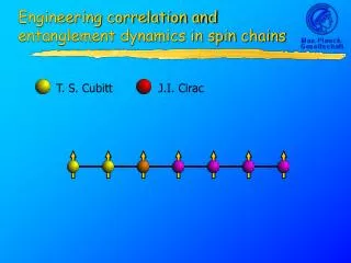
T. S. Cubitt J.I. Cirac Engineering correlation and entanglement dynamics in spin chains
T. S. Cubitt • Motivation and goals • Time evolution of a chain • Correlation and entanglement wave-packets • Engineering the dynamics: solitons etc. • Fermionic gaussian state formalism • Conclusions Engineering correlation and entanglement dynamics in spin chains J.I. Cirac
Many papers on correlations/entanglement of ground states • Fewer on time-dependent behaviour away from equilibrium • New experiments… • …motivate new theoretical studies of non-equilibrium behaviour. Conceptual motivation: new experiments
Many papers on correlations/entanglement of ground states. • Fewer on time-dependent behaviour away from equilibrium • In Phys. Rev. A 71, 052308 (2005), we used our entanglement rate equations to bound the time taken to entangle the ends of a length L chain. • Left open question of whether our pL lower bound is tight. • In J.Stat.Mech. 0504 (2005) p.010, Calabrese and Cardy investigated the time-evolution of block-entropy in spin chains. • Bravyi, Hastings and Verstraete (quant-ph/0603121)recently used Lieb-Robinson to prove tighter, linear bound. Existing results
“Traditional” solution to entanglement distribution:build a quantum repeater. • Getting to the ground state may be unrealistic. • Why not use non-equilibrium dynamics to distribute entanglement? • But a real quantum repeater involves particle interactions, e.g. atoms in cavities. • Alternative (e.g. Popp et al., Phys. Rev. A 71, 042306 (2005)): use entanglement in ground state: Practical motivation: quantum repeaters
T. S. Cubitt J.I. Cirac • Motivation and goals • Time evolution of a chain • Correlation and entanglement wave-packets • Engineering the dynamics: solitons etc. • Fermionic gaussian state formalism • Conclusions Engineering correlation and entanglement dynamics in spin chains
As an exactly-solvable example, we take the XY model… anisotropy magnetic field …and start it in some separable state, e.g. all spins +. Time evolution of a spin chain (1)
Fourier: • Solved by a well-known sequence of transformations: • Bogoliubov: • Jordan-Wigner: Time evolution of a spin chain (2)
Initial state N|+i… …is vacuum of the cl=zj-l operators. • Wick’s theorem: all correlation functions hxm…pni of the ground state of a free-fermion theory can be re-expressed in terms of two-point correlation functions. • Our initial state is a fermionic Gaussian state: it is fully specified by its covariance matrix: Time evolution of a spin chain (3)
Hamiltonian… …is quadratic in x and p. Gaussian state stays gaussian under gaussian evolution. • From Heisenberg equations, can show that time evolution under any quadratic Hamiltonian: corresponds to an orthogonal transformation of the covariance matrix: Time evolution of a spin chain (4)
Initial state is a fermionic gaussianstate in xl and pl. • Time-evolution is a fermionic gaussianoperation in xk and pk. • Fourier and Bogoliubov transformations are gaussian: Connected by Fourier and Bogoliubov transformations Time evolution of a spin chain (5)
xk , pk xk , pk xk , pk xk , pk xk , pkxl , pl time-evolve initial state • Putting everything together: Time evolution of a spin chain (phew!)
T. S. Cubitt J.I. Cirac • Motivation and goals • Time evolution of a chain • Correlation and entanglement wave-packets • Engineering the dynamics: solitons etc. • Fermionic gaussian state formalism • Conclusions Engineering correlation and entanglement dynamics in spin chains
We can get string correlationshanzlbmifor free… • Equations are very familiar: wave-packets with envelopeS propagating according to dispersion relation(). • Given directly by covariance matrixelements, e.g.: String correlations
Two-point connected correlation functions hznzmi - hznihzmi can also be obtained from the covariance matrix. • Again get wave-packets (3 of them) propagating according to dispersion relation(k). • Using Wick’s theorem: Two-point correlations
The relevant measure for entanglement distribution (e.g. in quantum repeaters) is the localisable entanglement (LE). • Definition: maximum entanglement between two sites (spins) attainable by LOCC on all other sites, averaged over measurement outcomes. • As with all operationally defined entanglement measures, LE is difficult to calculate in practice. • Best we can hope for is a lower bound. • Popp et al., Phys. Rev. A 71, 042306 (2005): LE is lower-bounded by any two-point connected correlation function. • In case you missed it: we’ve just calculated this! What about entanglement?
T. S. Cubitt J.I. Cirac • Motivation and goals • Time evolution of a chain • Correlation and entanglement wave-packets • Engineering the dynamics: solitons etc. • Fermionic gaussian state formalism • Conclusions Engineering correlation and entanglement dynamics in spin chains
In particular, around =1.1, =2.0 all three wave-packets in the two-point correlation equations are nearly identical • !localised packets propagate at well-defined velocity with minimaldispersion: “soliton-like” behaviour • In other parameter regimes: narrower wave-packets in nearly linear regions of dispersion relation • ! packets maintain their coherence as they propagate • In some parameter regimes: broadwave-packets and a highly non-linear dispersion relation • ! correlations rapidly disperse and disappear Correlation wave-packets
The system parameters and simultaneously control both the dispersion relation and form of the wave-packets. • In some parameter regimes: broadwave-packets and a highly non-linear dispersion relation • ! correlations rapidly disperse and disappear: (=10, =2) Correlation wave-packets (1)
In other parameter regimes, all three wave-packets in the two-point correlation equations are nearly identical • !localised packets propagate at well-defined velocity with minimaldispersion: “soliton-like” behaviour: (=1.1, =2) Correlation/entanglement solitons
If the parameters are changed with time, • ! Effective evolution under time-averaged Hamiltonian. • In general, time-ordering is essential. • But if parameters change slowly, dropping it gives reasonable approximation. • If we stay within “soliton” regime, adjusting the parameters only changes gradient of the dispersion relation, without significantly affecting its curvature. • ! Can speed up and slow down the “solitons”. Controlling the soliton velocity (1)
Starting from =1.1, =2.0 and changing at rate +0.01: Controlling the soliton velocity (2)
What happens if we do the opposite: rapidly change parameters from one regime to another? • Can calculate this analytically using same machinery as before. • Resulting equations are uglier, but still separate into terms describing multiple wave-packets propagating and interfering. Get four types of behaviour for the wave-packets: • Evolution according to 1 for t1, then 2 • Evolution according to 1 for t1, then -2 • Evolution according to 1untilt1, no evolution thereafter • Evolution according to 2starting att1 • Choose parameters so that “frozen” packets remain relatively coherent, whilst others rapidly disperse. “Quenching” correlations (1)
Choose parameters so that “frozen” packets remain relatively coherent, whilst others rapidly disperse. • ! can move correlations/entanglement to desired location, then “quench” system to freeze it there. • E.g. =0.9, =0.5 changed to =0.1, =10.0 at t1=20.0: “Quenching” correlations (2)
T. S. Cubitt J.I. Cirac • Motivation and goals • Time evolution of a chain • Correlation and entanglement wave-packets • Engineering the dynamics: solitons etc. • Fermionic gaussian state formalism • Conclusions Engineering correlation and entanglement dynamics in spin chains
There is another LE bound we can calculate… • Not a covariance matrix element because of |*i. • Recall concurrence: • Localisable concurrence: What about entanglement? (2)
Recap of gaussian state formalism… • What’s missing? A fermionicphase-space representation. Bosonic case Fermionic case • Operators a, aycommute • Operators c, cyanti-commute • States specified by symmetric covariance matrix • States specified by antisymmetric covariance matrix • Gaussian operations $symplectic transformations of • Gaussian operations $orthogonal transformations of Fermionic gaussian formalism
For bosons… • Eigenstates of an are coherent states: an|i = n|i • Define displacement operators: D()|vaci = |i • Characteristic function for state is:() = tr(D() ) For fermions… • Try to define coherent states: cn|i = n|i… • …but hit up against anti-commutation:cncm|i = m n|i but cncm|i = -cmcn|i = -n m|i • Define gaussian state to have gaussian characteristic function: • Eigenvalues anti-commute!? Fermionic phase space (1)
Coherent states and displacement operators now work:cncm|i = -cmcn|i = -n m|i = m n|i = cncm|i • Characteristic function for a gaussian state is again gaussian: • Grassman calculus: • Solution: expand fermionic Fock space algebra to include anti-commuting numbers, or “Grassmann numbers”, n. • Grassman algebra:n m = -m n)n2=0; for convenience n cm = -cm n Fermionic phase space (2)
We will need another phase-space representation: the fermionic analogue of the P-representation. • Essentially, it is a (Grassmannian) Fourier transform of the characteristic function. • Useful because it allows us to write state in terms of coherent states: • For gaussian states: Fermionic phase space (3)
Finally, • Recall bound on localisable entanglement: • Substituting the P-representation for states and * :and expanding xnand pn in terms of cnand cn y, the calculation becomes simple since coherent states are eigenstates of c. • Not very useful since bound 0 in thermodynamic limit N 1. What about entanglement (3)
Already leading to new theoretical results, e.g.: • Michael Wolf has used fermionic gaussian states to prove an area law for a large class of fermionic systems, in arbitrary dimensions: Phys. Rev. Lett. 96, 010404 (2006) • However, experimentalists are starting to build atomic analogues of quantum optical setups: e.g. atom lasers, atom beam splitters. • Fermionic gaussian state formalism may become important as fermionic gaussian states and operations move into the lab. Fermionic phase space (4)
T. S. Cubitt J.I. Cirac • Motivation and goals • Time evolution of a chain • Correlation and entanglement wave-packets • Engineering the dynamics: solitons etc. • Fermionic gaussian state formalism • Conclusions Entanglement flow in multipartite systems
Have shown that correlation and entanglement dynamics in a spin chain can be described by simple physics: wave-packets. Correlation dynamics can be engineered: • Set parameters to produce “soliton-like” behaviour • Control “soliton” velocity by adjusting parameters slowly in time • Freeze correlations at desired location by quenching the system • Developed fermionic gaussian state formalism, likely to become more important as experimentalists are starting to do gaussian operations on atoms in the lab (atom lasers, atomic beam-splitters…). Conclusions