DATA STRUCTURE

1. DATA STRUCTURE Instructor: Dai Min Office: XNA602 Fall 2006

2. CHAPTER 4Graphs • Basic terminology • Graph Implementation • Graph Traversals • Minimal Cost Spanning Tree • Shortest Path Problem

3. 4.1Graphs 1) Definition • A graph G consists of two sets • a finite, nonempty set of vertices V(G) • a finite, possible empty set of edges E(G) • G(V,E) represents a graph • The number of vertices is written |V|, and the number edges is written |E|. • General graphs differ from trees • need not have a root node • no implicit parent-child relationship • may be several (or no) paths from one vertex to another.

4. An undirected graph is one in which the pair of vertices in a edge is unordered, (v0, v1) = (v1,v0) • A directed graph is one in which each edge is a directed pair of vertices, <v0, v1> != <v1,v0> • A complete graph is a graph that has the maximum number of edges • for undirected graph with n vertices, the maximum number of edges is n(n-1)/2 • for directed graph with n vertices, the maximum number of edges is n(n-1)

5. Examples for Graph V(G1)={0,1,2,3} E(G1)={(0,1),(0,2),(0,3),(1,2),(1,3),(2,3)} V(G2)={0,1,2,3,4,5,6} E(G2)={(0,1),(0,2),(1,3),(1,4),(2,5),(2,6)} V(G3)={0,1,2} E(G3)={<0,1>,<1,0>,<1,2>} V(G4)={0,1,2,3} E(G4)={<0,1>,<0,2>,<0,3>,<1,0>,<1,2>, <1,3>,<2,0>,<2,1>,<2,3>,<3,0>, <3,1>,<3,2>}

6. Adjacent and Incident • If (v0,v1) is an edge in an undirected graph, • v0 and v1 are adjacent • The edge (v0, v1) is incident on vertices v0 and v1 • If <v0, v1> is an edge in a directed graph • v0 is adjacent to v1, and v1 is adjacent from v0 • The edge <v0, v1> is incident on v0 and v1 • Weighted digraph:there is some “cost” or “weight” associated with each edge. • A subgraph of G is a graph G’ such that V(G’) is a subset of V(G) and E(G’) is a subset of E(G)

7. The degree of a vertex is the number of edges incident to that vertex • For directed graph, • the in-degree of a vertex v is the number of edges that have v as the head • the out-degree of a vertex v is the number of edges that have v as the tail • if di is the degree of a vertex i in a graph G with n vertices and e edges, the number of edges is

8. undirected graph degree 0 3 0 2 1 2 1 2 3 3 3 3 3 6 5 4 3 3 1 1 1 1 0 in:1, out: 1 directed graph in-degree out-degree in: 1, out: 2 1 in: 1, out: 0 2

9. A path from vertex vp to vq in a graph G is a sequence of vertices, vp, vi1, vi2, ..., vin, vq, such that (vp, vi1), (vi1, vi2), ..., (vin, vq) are edges in an graph. • The length of a path is the number of edges on it • A simple path is a path in which all vertices, except possibly the first and the last, are distinct • A cycle is a simple path in which the first and the last vertices are the same

10. 2）ADT of Graph ADT Graph { Objects:a nonempty set of vertices and a set of edges, where each edge is a pair of vertices Functions: for all graphGraph, v, v1 and v2Vertices Graph Create()::=return an empty graph Graph DeleteEdge(graph, v1, v2)::=return a graph in which the edge (v1, v2) is removed Boolean IsEmpty(graph)::= if (graph==empty graph) return TRUE; else return FALSE …… } ADT Graph

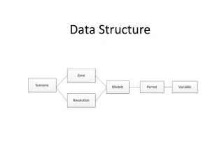
11. 4.2 Graph Implementation 4.2.1 Adjacency Matrix 1) Definition:Let G=(V,E) be a graph with n vertices. • The adjacency matrix of G is a two-dimensional n by n array, say A[n][n] • For a weighted digraph

12. Examples for Adjacency Matrix • The adjacency matrix for an undirected graph is symmetric; the adjacency matrix for a digraph need not be symmetric

13. For a weighted digraph the weight of the edge from vertex i to vertex j is used instead of 1 in the adjacency matrix.

14. 2) Merits of Adjacency Matrix • From the adjacency matrix, to determine the connection of vertices is easy • The degree of a vertex is • For a directed digraph, the sum of 1 (or true) in row i of the adjacency matrix is yields the out-degree of the ith vertex. • The sum of the entries in the ith column is its in-degree.

15. 3) Declaration #define MaxVNum 100 /*最大顶点数设为100*/ typedef XXX VertexType; /*顶点类型*/ typedef int EdgeType; /*边的权值设为整型*/ 邻接矩阵类型： typedef struct ArcCell { VertexType adj; InfoType *Info; // 存弧相关信息 } ArcCell, AdjMatrix[MaxVNum][MaxVNum] 图类型： typedef struct { VertexType vexs[MaxVNum]; /*顶点表*/ AdjMatrix arcs; /*邻接矩阵，即边表*/ int vexnum, arcnum; /*图的顶点数和边数*/ } Mgragh; /*Maragh是以邻接矩阵存储的图*/

16. 4) Create a Graph

17. CreateGraph (Maragh &ga) • { int i, j, k; float w; • scanf ( &ga.vexnum, &ga.arcnum); • for ( i=0; i <ga.vexnum ; i++) • ga->vexs[i]＝getchar(); /*读入顶点信息，建立顶点表*/ • for ( i=0; i < ga.vexnum ; i++) • for (j=0; j < ga.vexnum; j++) • ga->arcs[i][j]＝0; /*邻接矩阵初始化*/ • for ( k=0; k< ga.arcnum; k++) • { scanf (&v1, &v2, &w); /*读入一条边的顶点和权值*/ • i=LocateVex(ga,v1); j=LocateVex(ga,v2); • ga.arcs[i][j].adj ＝w; ga. arcs[j][i].adj＝w; • } • }

18. 4.2.2 Adjacency List • If a graph does not have many edges, the adjacency matrix will be sparse • such representation is a waste of space • use an array of pointers to linked row-lists • adjacency-list representation for digraphs.

19. 1) Adjacency List • Each row in adjacency matrix is represented as an adjacency list. • The graph is represented by an array or vector v[1], v[2],...,v[n], one element for each vertex in the digraph. • Each v[i] stores the data stored in vertex i together with a linked list of the numbers of all vertices adjacent to vertex i.

20. Example

21. 2) Merits of Adjacency Matrix • degree of a vertexin an undirected graph • # of nodes in adjacency list • out-degreeof a vertex in a directed graph • # of nodes in its adjacency list • in-degreeof a vertex in a directed graph • traverse the whole data structure

22. a b c d 3 1 1 4 a b vexdata adjvex firstarc next 1 ^ c d 2 ^ G1 3 ^ 4 ^ • Inverse adjacency list

23. 3) Declaration ＃define MaxVerNum 100 /*最大顶点数为100*/ 邻接表类型 ： typedef struct ArcNode { int adjvex; /*邻接点域*/ InfoType *Info; /*表示边上信息的域info*/ struct ArcNode * next; /*指向下一个邻接点的指针域*/ } ArcNode ; 表头结点类型 ： typedef struct Vnode { VertexType vertex; /*顶点域*/ ArcNode * firstedge; /*边表头指针*/ } Vnode, AdjList [MaxVertexNum]; 图的类型 ： typedef struct { AdjList vertices; /*邻接表*/ int vexnum, arcnum; /*顶点数和边数*/ } ALGraph; /*ALGraph是以邻接表方式存储的图类型*/

24. 4.3 Graph Traversals • Some applications require visiting every vertex in the graph exactly once. • The application may require that vertices be visited in some special order based on graph topology. • depth-first search • breadth-first search

25. 4.3.1Depth-First Search 1) Basic Idea： • Start from a given vertex v and visit it. • Visit the first neighbor, w, of v. Then visit the first neighbor of w that has not already been visited, etc. • If a node with no unexamined neighbors, then backup to the last visited node and examine its remaining neighbors. • The search continues until all nodes of the graph have been examined.

26. V1 V1 V2 V3 V2 V3 V4 V5 V6 V7 V4 V5 V6 V7 V8 V8 Example: V1 V2 V4  V8 V5 V6 V3 V7 V1 V2 V4  V8 V3 V6 V7 V5

27. Example: A、B、D、C

28. 2) Algorithm • Difficulties： • How to determine whether v has been visited? • How to search the neighbor of v？ • Solutions： • Using an array visited[n]. When i-thvertex has been visited, visited[i]=1. • Varying by different data structure： • Adjacency Matrix： • Adjacency List：

29. DFS uses backtracking. Recursion is a natural technique for such problems. • a stack is automatically maintained to make backtracking possible. • DFS • Visit the start vertex v. • For each vertex w adjacent to v do: • If w has not been visited, apply the depth-first search algorithm with w as the start vertex. 

30. 开始 开始 访问Vi,置标志 标志数组初始化 求Vi邻接点 Vi=1 N 有邻接点W N Vi访问过 Y Y 结束 Y W访问过 DFS N Vi=Vi+1 N 求下一邻接点 W Vi Vi==Vexnums Y DFS 结束

31. 3) Algorithm Analysis Let G=(V,E) be a graph with n vertices and e edges. • Adjacency list: O(n+e)。 • Adjacency matrix:O(n2)。

32. 4.3.2 Breadth-First Search 1) Basic Idea： • Start from a given vertex v and visit it. • Visit all neighbors of v. • Then visit all neighbors of first neighbor w of v. • Then visit all neighbors of second neighbor x of v, etc.

33. V1 V1 V2 V3 V2 V3 V4 V5 V6 V7 V4 V5 V6 V7 V8 V8 Example: BFS：V1 V2 V3  V4 V5 V6 V7 V8 BFS：V1 V2 V3  V4 V6 V7 V8 V5

34. Example: BFS：A、B、C、D

35. 2) Algorithm • BFS visits nodes level by level. • While visiting each node on a given level, • store it • so that, we can return to it after completing this level • so that nodes adjacent to it can be visited. • Because the first node visited on a given level should be the first one to which we return, a queue is an appropriate data structure for storing the nodes. 

36. BFS • Visit the start vertex v. • Initialize a queue to contain only the start vertex. • While the queue is not empty do: • Remove a vertex v from the queue. • For all vertices w adjacent to v do: • If w has not been visited then i. Visit w. ii. Add w to the queue.

37. 开始 标志数组初始化 Vi=1 N Vi访问过 Y BFS Vi=Vi+1 N Vi==Vexnums Y 结束 • Graph Traversal • Initialize an array or vector unvisited: visited[i] false for each vertex i. • While some element of unvisited is false, do: • Select an unvisited vertex v. • Use BFS or DFS to visit all vertices reachable from v.

38. 开始 访问Vi,置标志 初始化队列 Vi入队 Y 队列空吗 a N 访问W,置标志 队头V出队 结束 求V邻接点W W入队 N W存在吗 V下一邻接点W Y Y W访问过 N a BFS

39. 4.4 Spanning Trees 4.4.1 Connected Components • In an undirected graph G, two vertices, v0 and v1, are connected if there is a path in G from v0 to v1. • An undirected graph is connected if, for every pair of distinct vertices vi, vj, there is a path from vi to vj. • A connected component of an undirected graph is a maximal connected subgraph. • Any connected graph with n vertices must have at least n-1 edges.

40. A directed graph is strongly connected if there is a directed path from vi to vj and also from vj to vi. • A strongly connected component is a maximal subgraph that is strongly connected. • When graph G is connected, a depth first or breadth first search starting at any vertex will visit all vertices in G

41. 例 2 4 5 1 3 6 例 例 2 4 5 5 1 3 6 3 6 连通图 强连通图 非连通图 连通分量

42. 4.4.2 Minimal Cost Spanning Trees 1) Spanning Trees • A spanning tree is any tree that consists solely of edges in G and that includes all the vertices. • E(G): T (tree edges) + N (nontree edges) where T: set of edges used during search N: set of remaining edges • A spanning tree is a minimal subgraph, G’, of G such that V(G’)=V(G) and G’ is connected.

43. Examples of Spanning Tree 0 0 0 0 1 2 1 2 1 2 1 2 3 3 3 3 G1 Possible spanning trees

44. Either DFS or BFS can be used to create a spanning tree • When DFS is used, the resulting spanning tree is known as a depth first spanning tree • When BFS is used, the resulting spanning tree is known as a breadth first spanning tree • While adding a nontree edge into any spanning tree, this will create a cycle

45. V1 V1 V2 V3 V2 V3 V4 V5 V6 V7 V4 V5 V6 V7 V8 V1 V8 V1 V2 V3 V1 V2 V3 V2 V3 V4 V6 V4 V5 V6 V7 V4 V5 V6 V7 V8 V7 V8 V8 V5 depth first spanning tree breadth first spanning tree Example DFS：V1 V2 V4  V8 V5 V3 V6 V7 BFS：V1 V2 V3  V4 V5 V6 V7 V8

46. A B C D E F G H I K D A J L M L C F E depth first spanning forest M B J G K I H Example

47. Select n-1 edges from a weighted graph of n vertices with minimal cost. 2) Minimal Cost Spanning Trees • The cost of a spanning tree of a weighted undirected graph is the sum of the costs of the edges in the spanning tree • A minimal cost spanning tree is a spanning tree of least cost • Three different algorithms can be used • Prim • Kruskal

48. Greedy Strategy • An optimal solution is constructed in stages • At each stage, the best decision is made at this time • Since this decision cannot be changed later, we make sure that the decision will result in a feasible solution • Typically, the selection of an item at each stage is based on a least cost or a highest profit criterion

49. Prim’s Idea • Let the minimum cost spanning tree be T={U,TE } and U=V, TE  E. Initially, U={u0}, TE=; • Adding edge and vertices to T one at a time. • Select the least cost edge (u,v) that u∈U and v U. Adding v to U and (u,v) to TE; • It continue, until n-1 edges have been selected and U=V

50. 1 5 6 1 1 1 2 4 5 1 5 1 3 3 2 3 3 4 6 4 6 5 6 6 1 1 1 1 2 4 1 1 5 2 4 4 5 3 3 2 3 3 4 2 2 4 4 5 6 6 6 Examples for Prim’s Algorithm 1