Download
1 / 16
160 likes | 312 Views
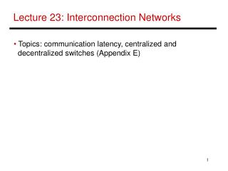
Lecture 23: Interconnection Networks. Topics: communication latency, centralized and decentralized switches (Appendix E). Topologies. Internet topologies are not very regular – they grew incrementally Supercomputers have regular interconnect topologies

E N D
Lecture 23: Interconnection Networks • Topics: communication latency, centralized and • decentralized switches (Appendix E)
Topologies • Internet topologies are not very regular – they grew • incrementally • Supercomputers have regular interconnect topologies • and trade off cost for high bandwidth • Nodes can be connected with • centralized switch: all nodes have input and output wires going to a centralized chip that internally handles all routing • decentralized switch: each node is connected to a switch that routes data to one of a few neighbors
Centralized Crossbar Switch P0 Crossbar switch P1 P2 P3 P4 P5 P6 P7
Centralized Crossbar Switch P0 P1 P2 P3 P4 P5 P6 P7
Crossbar Properties • Assuming each node has one input and one output, a • crossbar can provide maximum bandwidth: N messages • can be sent as long as there are N unique sources and • N unique destinations • Maximum overhead: WN2 internal switches, where W is • data width and N is number of nodes • To reduce overhead, use smaller switches as building • blocks – trade off overhead for lower effective bandwidth
Switch with Omega Network 000 P0 000 001 P1 001 010 P2 010 011 P3 011 100 P4 100 101 P5 101 110 P6 110 111 P7 111
Omega Network Properties • The switch complexity is now O(N log N) • Contention increases: P0 P5 and P1 P7 cannot • happen concurrently (this was possible in a crossbar) • To deal with contention, can increase the number of • levels (redundant paths) – by mirroring the network, we • can route from P0 to P5 via N intermediate nodes, while • increasing complexity by a factor of 2
Tree Network • Complexity is O(N) • Can yield low latencies when communicating with neighbors • Can build a fat tree by having multiple incoming and outgoing links P0 P1 P2 P3 P4 P5 P6 P7
Bisection Bandwidth • Split N nodes into two groups of N/2 nodes such that the • bandwidth between these two groups is minimum: that is • the bisection bandwidth • Why is it relevant: if traffic is completely random, the • probability of a message going across the two halves is • ½ – if all nodes send a message, the bisection • bandwidth will have to be N/2 • The concept of bisection bandwidth confirms that the • tree network is not suited for random traffic patterns, but • for localized traffic patterns
Distributed Switches: Ring • Each node is connected to a 3x3 switch that routes • messages between the node and its two neighbors • Effectively a repeated bus: multiple messages in transit • Disadvantage: bisection bandwidth of 2 and N/2 hops on • average
Distributed Switch Options • Performance can be increased by throwing more hardware • at the problem: fully-connected switches: every switch is • connected to every other switch: N2wiring complexity, • N2/4 bisection bandwidth • Most commercial designs adopt a point between the two • extremes (ring and fully-connected): • Grid: each node connects with its N, E, W, S neighbors • Torus: connections wrap around • Hypercube: links between nodes whose binary names differ in a single bit
Topology Examples Hypercube Grid Torus
Topology Examples Hypercube Grid Torus
k-ary d-cube • Consider a k-ary d-cube: a d-dimension array with k • elements in each dimension, there are links between • elements that differ in one dimension by 1 (mod k) • Number of nodes N = kd Number of switches : Switch degree : Number of links : Pins per node : Avg. routing distance: Diameter : Bisection bandwidth : Switch complexity : Should we minimize or maximize dimension?
k-ary d-Cube • Consider a k-ary d-cube: a d-dimension array with k • elements in each dimension, there are links between • elements that differ in one dimension by 1 (mod k) • Number of nodes N = kd (with no wraparound) Number of switches : Switch degree : Number of links : Pins per node : N Avg. routing distance: Diameter : Bisection bandwidth : Switch complexity : d(k-1)/2 2d + 1 d(k-1) Nd 2wkd-1 2wd (2d + 1)2 Should we minimize or maximize dimension?
Title • Bullet