Turbulent combustion (Lecture 1)
480 likes | 878 Views
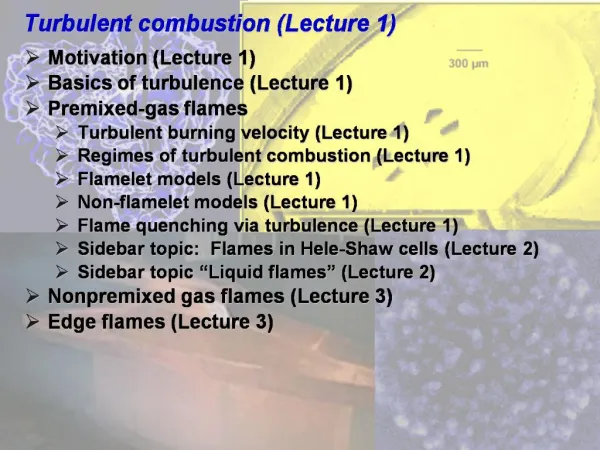
Turbulent combustion (Lecture 1). Motivation (Lecture 1) Basics of turbulence (Lecture 1) Premixed-gas flames Turbulent burning velocity (Lecture 1) Regimes of turbulent combustion (Lecture 1) Flamelet models (Lecture 1) Non-flamelet models (Lecture 1)

Turbulent combustion (Lecture 1)
E N D
Presentation Transcript
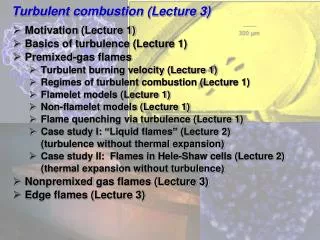
Turbulent combustion (Lecture 1) • Motivation (Lecture 1) • Basics of turbulence (Lecture 1) • Premixed-gas flames • Turbulent burning velocity (Lecture 1) • Regimes of turbulent combustion (Lecture 1) • Flamelet models (Lecture 1) • Non-flamelet models (Lecture 1) • Flame quenching via turbulence (Lecture 1) • Case study I: “Liquid flames” (Lecture 2) (turbulence without thermal expansion) • Case study II: Flames in Hele-Shaw cells (Lecture 2) (thermal expansion without turbulence) • Nonpremixed gas flames (Lecture 3) • Edge flames (Lecture 3) AME 514 - Spring 2013 - Lecture 7
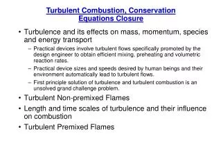
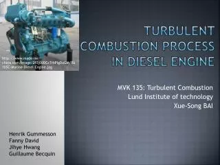
Motivation • Almost all flames used in practical combustion devices are turbulent because turbulent mixing increases burning rates, allowing more power/volume • Even without forced turbulence, if the Grashof number gd3/2 is larger than about 106 (g = 103 cm/s2, ≈ 1 cm2/s d > 10 cm), turbulent flow will exist due to buoyancy • Examples • Premixed turbulent flames • Gasoline-type (spark ignition, premixed-charge) internal combustion engines • Stationary gas turbines (used for power generation, not propulsion) • Nonpremixed flames • Diesel-type (compression ignition, nonpremixed-charge) internal combustion engines • Gas turbines • Most industrial boilers and furnaces AME 514 - Spring 2013 - Lecture 7
Basics of turbulence • Good reference: Tennekes: “A First Course in Turbulence” • Job 1: need a measure of the strength of turbulence • Define turbulence intensity (u’) as rms fluctuation of instantaneous velocity u(t) about mean velocity ( ) • Kinetic energy of turbulence = mass*u’2/2; KE per unit mass (total in all 3 coordinate directions x, y, z) = 3u’2/2 AME 514 - Spring 2013 - Lecture 7
Basics of turbulence • Job 2: need a measure of the length scale of turbulence • Define integral length scale (LI) as • A measure of size of largest eddies • Largest scale over which velocities are correlated • Typically related to size of system (tube or jet diameter, grid spacing, …) Here the overbars denote spatial (not temporal) averages • A(r) is the autocorrelation function at some time t • Note A(0) = 1 (fluctuations around the mean are perfectly correlated at a point) • Note A(∞) = 0 (fluctuations around the mean are perfectly uncorrelated if the two points are very distant) • For truly random process, A(r) is an exponentially decaying function A(r) = exp(-r/LI) AME 514 - Spring 2013 - Lecture 7
Basics of turbulence • In real experiments, generally know u(t) not u(x) - can define time autocorrelation function A(x,) and integral time scale I at a point x Here the overbars denote temporal (not spatial) averages • With suitable assumptions LI = (8/π)1/2u’I • Define integral scale Reynolds number ReL u’LI/ ( = kinematic viscosity) • Note generally ReL ≠ Reflow = Ud/; typically u’ ≈ 0.1U, LI ≈ 0.5d, thus ReL ≈ 0.05 Reflow AME 514 - Spring 2013 - Lecture 7
nonlinear term Basics idea of turbulence • Large scales • Viscosity is unimportant (high ReL) - inertial range of turbulence • Through nonlinear interactions of large-scale features (e.g. eddies), turbulent kinetic energy cascades down to smaller scales • Interaction is NOT like linear waves: (e.g. waves on a string) that can pass through each other without changing or interacting in an irreversible way • Interaction is described by inviscid Navier-Stokes equation + continuity equation • Smaller scales: viscosity dissipates the KE generated at larger scales • Steady-state: rate of energy generation at large scales = rate of dissipation at small scales • Example: stir water in cup at large scale, but look later and see small scales - where did they come from??? AME 514 - Spring 2013 - Lecture 7
Energy dissipation • Why is energy dissipated at small scales? • Viscous term in NS equation (2u) scales as u’/(x)2, convective term (u)u as (u’)2/x, ratio convective / viscous ~ u’x/ = Rex - viscosity more important as Re (thus x) decreases • Define energy dissipation rate () as energy dissipated per unit mass (u’)2 per unit time (I) by the small scales • ~ (u’)2/I ~ (u’)2/(LI/u’) = C(u’)3/LI (units Watts/kg = m2/s3) • With suitable assumptions C = 3.1 • Note to obtain u’/SL = 10 for stoich. HC-air (SL = 40 cm/s) with typical LI = 5 cm, ≈ 4000 W/kg • Is this a lot of power? • If flame propagates at speed ST ≈ u’ across a distance LI, heat release per unit mass is YfQR and the time is LI/ST, thus heat release per unit mass per unit time is YfQRST/LI ≈ (0.068)(4.5 x 10⁷ J/kg)(4 m/s)/(0.05 m) ≈ 2.4 x 10⁸ W/kg • Ratio of power required to sustain turbulence (4000 W/kg) to attainable heat release rate ≈ 1.6 x 10⁻⁵ • Also: turbulent kinetic energy (not power) / heat release (not rate) = (3/2 u’2)/YfQR ≈ 8 x 10⁻⁶ ! • Answer: NO, very little power (or energy) AME 514 - Spring 2013 - Lecture 7
Kolmogorov universality hypothesis (1941) • In inertial range of scales, the kinetic energy (E) per unit mass per wavenumber (k) (k = 2π/, = wavelength) depends only on k and • Use dimensional analysis, E = (m/s)2/(1/m) = m3/s2, k = m-1 • E(k) ~ akb or m3/s2 ~ (m2/s3)a(1/m)b a = 2/3, b = -5/3 • E(k) = 1.62/3k-5/3 (constant from experiments or numerical simulations) (e.g. C = 1.606, Yakhot and Orzag, 1986) • Total kinetic energy (K) over a wave number range (k1 < k < k2) • Characteristic intensity at scale L = u’(k) = (2K/3)1/2 = 0.6871/3L1/3 • Cascade from large to small scales (small to large k) ends at scale where dissipation is important • Smallest scale in the turbulent flow • This scale (Kolmogorov scale) can depend only on and • Dimensional analysis: wave number kKolmogorov ~ (/3)1/4 or length scale LK = C(3/)1/4, C ≈ 11 • LK/LI = C(3/)1/4/LI = C(3/(3.1u’3/LI))1/4/LI = 14 (u’LI/)-3/4= 14 ReL-3/4 • Time scale tK ~ LK/u’(LK) ~ (/)1/2 AME 514 - Spring 2013 - Lecture 7
Kolmogorov universality hypothesis (1941) AME 514 - Spring 2013 - Lecture 7
There are three types of turbulent eddies large entrainment eddies inertial-range eddies dissipation-scale eddies K. Nomura, UCSD S. Tieszen, Sandia (Diagram courtesy A. Kerstein, Sandia National Labs) AME 514 - Spring 2013 - Lecture 7
Application of Kolmogorov scaling • Taylor scale (LT): scale at which average strain rate occurs • LT u’/(mean strain) • LT~ u’/(tK)-1 ~ u’/((/)1/2)-1 ~ u’1/2/(u’3/LI)1/2 ~ LIReL-1/2 • With suitable assumptions, mean strain ≈ 0.147(/)1/2 • Turbulent viscosity T • Molecular gas dynamics: ~ (velocity of particles)(length particles travel before changing direction) • By analogy, at scale k, T(k) ~ u’(k)(1/k) • Total effect of turbulence on viscosity: at scale LI, T ~ u’LI • Usually written in the form T = CK2/, C = 0.084 • OrT/ = 0.061 ReL • Turbulent thermal diffusivity T = T/PrT • Pr goes from molecular value (gases ≈ 0.7, liquids 10 - 10,000; liquid metals 0.05) at ReL = 0 to PrT ≈ 0.72 as ReL ∞ (Yakhot & Orzag, 1986) • T/ = 0.042 ReL as ReL ∞ AME 514 - Spring 2013 - Lecture 7
Turbulent premixed combustion - intro • Study of premixed turbulent combustion is important because • Turbulence increases mean flame propagation rate (ST) and thus mass burning rate (= ST Aprojected) • If this trend increased ad infinitum, arbitrarily lean mixtures (low SL) could be burned arbitrarily fast by using sufficiently high u’ ...but too high u' leads to extinction - nixes that idea • Current theories don't agree with experiments ...and don't agree with each other • Numerical simulations difficult at high u'/SL (>10) • Applications to • Auto engines • Gas turbine designs - possible improvements in emission characteristics with lean premixed combustion compared to non-premixed combustion (remember why?) AME 514 - Spring 2013 - Lecture 7
Bradley et al. (1992) • Compilation of data from many sources = ST/SL = u’/SL AME 514 - Spring 2013 - Lecture 7
Turbulent burning velocity • Experimental results shown in Bradley et al. (1992) smoothed data from many sources, e.g. fan-stirred bomb AME 514 - Spring 2013 - Lecture 7
Bradley et al. (1992) … and we are talking MAJOR smoothing! AME 514 - Spring 2013 - Lecture 7
Turbulent burning velocity • Models of premixed turbulent combustion don’t agree with experiments nor each other! AME 514 - Spring 2013 - Lecture 7
Modeling of premixed turbulent flames • Models often don’t agree well with experiments • Most model employ assumptions not satisfied by real flames, e.g. • Adiabatic (sometimes ok) • Homogeneous, isotropic turbulence over many LI(never ok) • Low Ka or high Da (thin fronts) (sometimes ok) • Lewis number = 1 (sometimes ok, e.g. CH4-air) • Constant transport properties (never ok, ≈ 25x increase in and across front!) • u’ doesn’t change across front (never ok, thermal expansion across flame generates turbulence) (but viscosity increases across front, decreases turbulence, sometimes almost cancels out) • Constant density (never ok!) AME 514 - Spring 2013 - Lecture 7
Characteristics of turbulent flames • Most important property: turbulent flame speed (ST) • Most models based on physical models of Damköhler (1940) • Behavior depends on Karlovitz number (Ka) • Kolmogorov turbulence: u = u’; L = LT = • Alternatively, Ka = (/LK)2 ~ (SL/)/(ReL-3/4LI)2 ~ ReL-1/2(u’/SL)2 - same scaling results based on length scales • Sometimes Damköhler number (Da) is reported instead • Da1 = I/chem~ (LI/u’)/(/SL2) ~ ReL(u’/SL)-2 • Da2 = Taylor/chem~ (ReL-1/2LI/u’)/(/SL2) ~ ReL1/2(u’/SL)-2 ~ 1/Ka • Low Ka: “Huygens propagation,” thin fronts that are wrinkled by turbulence but internal structure is unchanged • High Ka: Distributed reaction zones, broad fronts Defined using cold-gas viscosity AME 514 - Spring 2013 - Lecture 7
Characteristics of turbulent flames AME 514 - Spring 2013 - Lecture 7
Turbulent combustion regimes (Peters, 1986) Ka = Re1/2 Distributed reaction zones “Broadened” flames (Ronney & Yakhot, 1992) = u’/SL Laminar flames = LI/ = LI(SL/) = ReL/(u’/SL) AME 514 - Spring 2013 - Lecture 7
Turbulent combustion regimes • Comparison of flamelet and distributed combustion (Yoshida, 1988) Flamelet: temperature is either T∞ or Tad, never between, and probability of product increases through the flame Distributed: significant probability of temperatures between T∞ or Tad, probability of intermediate T peaks in middle of flame AME 514 - Spring 2013 - Lecture 7
Flamelet modeling • Damköhler (1940): in Huygens propagation regime, flame front is wrinkled by turbulence but internal structure and SL are unchanged • Propagation rate ST due only to area increase via wrinkling: ST/SL = AT/AL AME 514 - Spring 2013 - Lecture 7
Flamelet modeling • Low u’/SL: weakly wrinkled flames • ST/SL = 1 + (u’/SL)2 (Clavin & Williams, 1979) - standard for many years • Actually Kerstein and Ashurst (1994) showed this is valid only for periodic flows - for random flows ST/SL - 1 ~ (u’/SL)4/3 • Higher u’/SL: strongly wrinkled flames • Schelkin (1947) - AT/AL estimated from ratio of cone surface area to base area; height of cone ~ u’/SL; result • Other models based on fractals, probability-density functions, etc., but mostly predict ST/SL ~ u’/SL at high u’/SL with the possibility of “bending” or quenching at sufficiently high Ka ~ (u’/SL)2 AME 514 - Spring 2013 - Lecture 7
Flamelet modeling • Many models based on “G-equation” (Kerstein et al. 1987) • Any curve of G = C is a flame front (G < C burned; G > C burned) • Flame advances by self-propagation and advances or retreats by convection AME 514 - Spring 2013 - Lecture 7
Flamelet modeling • G-equation formulation, renormalization group (Yakhot, 1988) (successive scale elimination); invalid (but instructive) derivation: AME 514 - Spring 2013 - Lecture 7
Fractal models of flames • What is the length (L) is the coastline of Great Britain? Depends on measurement scale: L(10 miles) < L(1 mile) • Plot Log(L) vs. Log(measurement scale); if it’s a straight line, it’s a fractal with dimension (D) = 1 - slope • If object is very smooth (e.g. circle), D = 1 • If object has self-similar wrinkling on many scales, D > 1 - expected for flames since Kolmogorov turbulence exhibits scale-invariant properties • If object is very rough, D 2 • If object 3D, everything is same except length area, D D + 1 (space-filling surface: D 3) Generic 2D object 3D flame surface AME 514 - Spring 2013 - Lecture 7
Fractal models of flames • Application to flames (Gouldin, 1987) • Inner (small-scale) and outer (large-scale) limits (“cutoff scales”) • Outer: LI; inner: LK or LG (no clear winner…) • LG = “Gibson scale,” where u’(LG) = SL • Recall u’(L) ~ 1/3L1/3, thus LG ~ SL3/ • Since ~ u’3/LI thus LG ~ LI(SL/u’)3 • ST/SL = AT/AL = A(Linner)/A(Louter) • For 3-D object, A(Linner)/A(Louter) = (Louter/Linner)2-D • What is D? Kerstein (1988) says it should be 7/3 for a flame in Kolmogorov turbulence (consistent with experiments), but Haslam & Ronney (1994) show it’s 7/3 even in non-Kolmogorov turbulence! • With D = 7/3, Linner = LK, ST/SL = (LK/LI)2-7/3 ~ (ReL-3/4)-1/3 ~ ReL1/4 • With D = 7/3, Linner = LG, ST/SL = (LG/LI)2-7/3 ~ (u’/SL)-3)-1/3 ~ u’/SL • Consistent with some experiments (like all models…) AME 514 - Spring 2013 - Lecture 7
Effects of thermal expansion • Excellent review of flame instabilities: Matalon, 2007 • Thermal expansion across flame known to affect turbulence properties, thus flame properties • Exists even when no forced turbulence - Darrieus-Landau instability - causes infinitesimal wrinkle in flame to grow • Some models (e.g. Pope & Anand, 1987) predict thermal expansion decreases ST/SL for fixed u’/SL but most predict an increase Williams, 1985 Bernoulli: P+1/2u2 = const Aflame , u , P Aflame, u, P FLOW Aflame , u , P Aflame, u, P AME 514 - Spring 2013 - Lecture 7
Effects of thermal expansion • Byckov (2000): • Same as Yakhot (1988) if no thermal expansion ( = 1) • Also says for any , if u’/SL = 0 thenST/SL = 1; probably not true AME 514 - Spring 2013 - Lecture 7
Effects of thermal expansion • Cambray and Joulin (1992): one-scale (not really turbulent) flow with varying thermal expansion = 1-1/ • ST/SL increases as increases (more thermal expansion) • If ≠ 0, then ST/SLdoes not go to 1 as u’/SL goes to zero - inherent thermal expansion induced instability and wrinkling causes ST/SL > 1 even at u’/SL = 0 • Effect of expansion-induced wrinkling decreases as u’/SL AME 514 - Spring 2013 - Lecture 7
Effects of thermal expansion • Time-dependent computations in decaying turbulence suggest • Early times, before turbulence decays, turbulence dominates • Late times, after turbulence decays, buoyancy dominates • Next lecture: thermal expansion effects on ST with no ‘turbulence’, and turbulence effects on ST with no thermal expansion Boughanem and Trouve, 1998 Initial u'/SL = 4.0 (decaying turbulence); integral-scale Re = 18 = ∞/f - 1 Before turbulence decays - ST/SL is independent of density ratio Total reaction rate / reaction rate of flat steady flame More or less = ST/SL Well after initial turbulence decays - ST/SL depends totally on density ratio Time / turbulence integral time scale AME 514 - Spring 2013 - Lecture 7
Buoyancy effects • Upward propagation: buoyantly unstable, should increase ST compared to no buoyancy effects • Buoyancy affects largest scales, thus scaling of buoyancy effects should depend on integral time scale / buoyant time scale = (LI/u’)/(LI/g)1/2 = (gLI/u’2)1/2 = (SL/u’)(gLI/SL2)1/2 • Libby (1989) (g > 0 for upward propagation) • No systematic experimental test to date • Lewis (1970): experiments on flames in tubes in a centrifugal force field (50 go < g < 850 go), no forced turbulence: ST ~ g0.387, almost independent of pressure - may be same as S ~ g1/2 AME 514 - Spring 2013 - Lecture 7
Effects of buoyancy • Time-dependent computations in decaying turbulence suggest • Early times, before turbulence decays, turbulence dominates • Late times, after turbulence decays, buoyancy dominates - upward propagating: higher ST/SL; downward: almost no wrinkling, ST/SL ≈ 1 Boughanem and Trouve, 1998 Initial u'/SL = 4.0 (decaying turbulence); integral-scale Re = 18 Buoyancy parameter: Ri = g∞/SL3 Before turbulence decays - ST/SL is independent of buoyancy Total reaction rate / reaction rate of flat steady flame More or less = ST/SL Well after initial turbulence decays - ST/SL depends totally on buoyancy Time / turbulence integral time scale AME 514 - Spring 2013 - Lecture 7
Lewis number effects • Turbulence causes flame stretch & curvature • Since both + and - curved flamelets exist, effects nearly cancel (Rutland & Trouve, 1993) • Mean flame stretch is biased towards + stretch - benefits flames in low-Le mixtures • H2-air: extreme case, lean mixtures have cellular structures similar to flame balls - “Pac-Man combustion” • Causes change in behavior at 8% - 10% H2, corresponding to ≈ 0.25 (Al-Khishali et al., 1983) - same as transition from flame ball to continuous flames in non-turbulent mixtures AME 514 - Spring 2013 - Lecture 7
Distributed combustion modeling • Much less studied than flamelet combustion • Damköhler (1940): A ≈ 0.25 (gas); A ≈ 6.5 (liquid) • Assumption T ≈ L probably not valid for high ; recall …but probably ok for small • Example: 2 equal volumes of combustible gas with E = 40 kcal/mole, 1 volume at 1900K, another at 2100K (1900) ~ exp(-40000/(1.987*1900)) = 3.73 x 10⁴ (2100) ~ exp(-40000/(1.987*2100)) = 1.34 x 10⁴ Average = 2.55 x 10⁴, whereas (2000) = 2.2 x 10⁴ (16% difference)! Averaging over ±5% T range gives 16% error! AME 514 - Spring 2013 - Lecture 7
Distributed combustion modeling • Pope & Anand (1984) Constant density, 1-step chemistry, ≈ 12.3: ST/SL ≈ 0.3 (u’/SL)[0.64 + log10(ReL) - 2 log10(u’/SL)] - Close to Damköhler (1940) (?!) for relevant ReL AME 514 - Spring 2013 - Lecture 7
Distributed combustion modeling • When applicable? T ≥ LI • T ≈ 6T/ST (Ronney & Yakhot, 1992), ST/SL ≈ 0.25 ReL1/2 Ka ≥ 0.037 ReL1/2(based on cold-gas viscosity) • Experiments (Abdel-Gayed et al., 1989) • Ka ≥ 0.3: “significant flame quenching within the reaction zone” - independent of ReL • Applicable range uncertain, but probably only close to quenching • Experiment - Bradley (1992) • ST/SL ≈ 5.5 Re0.13 - close to models over limited applicable range • Implications for “bending” • Flamelet models generally ST ~ u’ • Distributed combustion models generally ST ~ √u’ • Transition from flamelet to distributed combustion - possible mechanism for “bending” AME 514 - Spring 2013 - Lecture 7
“Broadened” flames • Ronney & Yakhot, 1992: If Re1/2 > Ka > 1, some but not all scales (i.e. smaller scales) fit inside flame front and “broaden” it since T > • Combine flamelet (Yakhot) model for large (wrinkling) scales with distributed (Damköhler) model for small (broadening) scales • Results show ST/SL“bending” and even decrease in ST/SL at high u’/SL as in experiments • Still no consideration of thermal expansion, etc. AME 514 - Spring 2013 - Lecture 7
Quenching by turbulence • Low Da / high Ka: “thin-flame” models fail • “Distributed” combustion • “Quenching” at still higher Ka • Quenching attributed to mass-extinguishment of flamelets by zero-mean turbulent strain ...but can flamelet quenching cause flame quenching? • Hypothetical system: flammable mixture in adiabatic channel with arbitrary zero-mean flow disturbance • 1st law: No energy loss from system adiabatic flame temperature is eventually reached • 2nd law: Heat will be transferred to unburned gas • Chemical kinetics: (T>TH) >> (TL) Propagating front will always exist (???) AME 514 - Spring 2013 - Lecture 7
Quenching by turbulence AME 514 - Spring 2013 - Lecture 7
Turbulent flame quenching in gases • "Liquid flame" experiments suggest flamelet quenching does not cause flame quenching • Poinsot et al. (1990): Flame-vortex interactions • Adiabatic: vortices cause temporary quenching • Non-adiabatic: permanent flame quenching possible • Giovangigli and Smooke (1992) no intrinsic flammability limit for planar, steady, laminar flames • So what causes quenching in “standard” experiments? • Radiative heat losses? • Ignition limits? AME 514 - Spring 2013 - Lecture 7
Turbulent flame quenching in gases • High Ka (distributed combustion): • Turbulent flame thickness (T) >> L • Larger T more heat loss (~ T), ST increases less heat loss more important at high Ka Kaq ≈ 0.038 ReL0.76 for typical LI = 0.05 m • Also: large T large ignition energy required Kaq ≈ 2.3 ReL-0.24 • 2 limit regimes qualitatively consistent with experiments AME 514 - Spring 2013 - Lecture 7
Turbulent flame quenching in gases AME 514 - Spring 2013 - Lecture 7
References Abdel-Gayed, R. G. and Bradley, D. (1985) Combust. Flame 62, 61. Abdel-Gayed, R. G., Bradley, D. and Lung, F. K.-K. (1989) Combust. Flame 76, 213. Al-Khishali, K. J., Bradley, D., Hall, S. F. (1983). "Turbulent combustion of near-limit hydrogen-air mixtures," Combust. Flame Vol. 54, pp. 61-70. Anand, M. S. and Pope, S. B. (1987). Combust. Flame 67, 127. H. Boughanem and A. Trouve (1998). Proc. Combust. Inst. 27, 971. Bradley, D., Lau, A. K. C., Lawes, M., Phil. Trans. Roy. Soc. London A, 359-387 (1992) Bray, K. N. C. (1990). Proc. Roy. Soc.(London) A431, 315. Bychov, V. (2000). Phys. Rev. Lett. 84, 6122. Cambray, P. and Joulin, G. (1992). Twenty-Fourth Symposium (International) on Combustion, Combustion Institute, Pittsburgh, p. 61. Clavin, P. and Williams, F. A. (1979). J. Fluid Mech. 90, 589. Damköhler, G. (1940). Z. Elektrochem. angew. phys. Chem 46, 601. Gouldin, F. C. (1987). Combust. Flame 68, 249. Kerstein, A. R. (1988). Combust. Sci. Tech. 60, 163. Kerstein, A. R. and Ashurst, W. T. (1992). Phys. Rev. Lett. 68, 934. Kerstein, A. R., Ashurst, W. T. and Williams, F. A. (1988). Phys. Rev. A., 37, 2728. Lewis, G. D. (1970). Combustion in a centrifugal-force field. Proc. Combust. Inst. 13, 625-629. AME 514 - Spring 2013 - Lecture 7
References Libby, P. A. (1989). Theoretical analysis of the effect of gravity on premixed turbulent flames, Combust. Sci. Tech. 68, 15-33. Matalon, M. (2007). Intrinsic flame instabilities in premixed and nonpremixed combustion. Ann. Rev. Fluid. Mech. 39, 163 - 191. Poinsot, T., Veyante, D. and Candel, S. (1990). Twenty-Third Symposium (International) on Combustion, Combustion Institute, Pittsburgh, p. 613. Pope, S. B. and Anand, M. S. (1984). Twentieth Symposium (International) on Combustion, Combustion Institute, Pittsburgh, p. 403. Peters, N. (1986). Twenty-First Symposium (International) on Combustion, Combustion Institute, Pittsburgh, p. 1231 Ronney, P. D. and Yakhot, V. (1992). Combust. Sci. Tech. 86, 31. Rutland, C. J., Ferziger, J. H. and El Tahry, S. H. (1990). Twenty-Third Symposium (International) on Combustion, Combustion Institute, Pittsburgh, p. 621. Rutland, C. J. and Trouve, A. (1993). Combust. Flame 94, 41. Sivashinsky, G. I. (1990), in: Dissipative Structures in Transport Processes and Combustion (D. Meinköhn, ed.), Springer Series in Synergetics, Vol. 48, Springer-Verlag, Berlin, p. 30. Yakhot, V. (1988). Combust. Sci. Tech. 60, 191. Yakhot, V. and Orzag, S. A. (1986). Phys. Rev. Lett. 57, 1722. Yoshida, A. (1988). Proc. Combust. Inst. 22, 1471-1478. AME 514 - Spring 2013 - Lecture 7