Download
1 / 28
360 likes | 853 Views
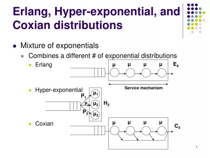
Erlang, Hyper-exponential, and Coxian distributions. Mixture of exponentials Combines a different # of exponential distributions Erlang Hyper-exponential Coxian. μ. μ. μ. E 4. μ. Service mechanism. μ 1. P 1. μ 2. H 3. P 2. P 3. μ 3. μ. μ. μ. μ. C 4.

E N D
Erlang, Hyper-exponential, and Coxian distributions • Mixture of exponentials • Combines a different # of exponential distributions • Erlang • Hyper-exponential • Coxian μ μ μ E4 μ Service mechanism μ1 P1 μ2 H3 P2 P3 μ3 μ μ μ μ C4
Erlang distribution: analysis 1/2μ 1/2μ • Mean service time • E[Y] = E[X1] + E[X2] =1/2μ + 1/2μ = 1/μ • Variance • Var[Y] = Var[X1] + Var[X2] = 1/4μ2 v +1/4μ2 = 1/2μ2 E2
Squared coefficient of variation: analysis constant exponential C2 • X is a constant • X = d => E[X] = d, Var[X] = 0 => C2 =0 • X is an exponential r.v. • E[X]=1/μ; Var[X] = 1/μ2 => C2 = 1 • X has an Erlang r distribution • E[X] = 1/μ, Var[X] = 1/rμ2 => C2 = 1/r • fX *(s) = [rμ/(s+rμ)]r Erlang 0 1 Hypo-exponential
Probability density function of Erlang r • Let Y have an Erlang r distribution • r = 1 • Y is an exponential random variable • r is very large • The larger the r => the closer the C2 to 0 • Er tends to infintiy => Y behaves like a constant • E5 is a good enough approximation
Generalized Erlang Er • Classical Erlang r • E[Y] = r/μ • Var[Y] = r/μ2 • Generalized Erlang r • Phases don’t have same μ … rμ rμ rμ Y … μ1 μ2 μr Y
Generalized Erlang Er: analysis • If the Laplace transform of a r.v. Y • Has this particular structure • Y can be exactly represented by • An Erlang Er • Where the service rates of the r phase • Are minus the root of the polynomials
Hyper-exponential distribution μ1 P1 • P1 + P2 + P3 +…+ Pk =1 • Pdf of X? μ2 X P2 . . Pk μk
Hyper-exponential distribution:1st and 2nd moments • Example: H2
Hyper-exponential: squared coefficient of variation • C2 = Var[X]/E[X]2 • C2 is greater than 1 • Example: H2 , C2 > 1 ?
Coxian model: main idea • Idea • Instead of forcing the customer • to get r exponential distributions in an Er model • The customer will have the choice to get 1, 2, …, r services • Example • C2 : when customer completes the first phase • He will move on to 2nd phase with probability a • Or he will depart with probability b (where a+b=1) a b
Coxian model μ2 μ3 μ4 μ1 a2 a3 a1 b1 b2 b3 μ1 b1 a1 b2 μ1 μ2 a1 a2 b3 μ1 μ2 μ3 a1 a2 a3 μ1 μ2 μ3 μ4
Coxian distribution: Laplace transform • Laplace transform of Ck • Is a fraction of 2 polynomials • The denominator of order k and the other of order < k • Implication • A Laplace transform that has this structure • Can be represented by a Coxian distribution • Where the order k = # phases, • Roots of denominator = service rate at each phase
Coxian model: conclusion • Most Laplace transforms • Are rational polynomials • => Any distribution can be represented • Exactly or approximately • By a Coxian distribution
Coxian model: dimensionality problem • A Coxian model can grow too big • And may have as such a large # of phases • To cope with such a limitation • Any Laplace transform can be approximated by a c • To obtain the unknowns (a, μ1, μ2) • Calculate the first 3 moments based on Laplace transform • And match these against those of the C2 a μ1 μ2 b=1-a
Rational polynomials approximated by Coxian-2 (C2) • The Laplace transforms of most pdfs • Have the following shape • Can be exactly represented by • A Coxian k (Ck) distribution • The # stages = the order of the denominator • Service rates given by the roots of the denominator • If k is very large => dimensionality problem • Solution: collapse the Ck into a C2 a μ1 μ2 b=1-a
3 moments method • The first way of obtaining the 3 unknowns (μ1μ2 a) • 3 moments method • Let m1, m2, m3 be the first three moments • of the distribution which we want to approximate by a C2 • The first 3 moments of a C2 are given by • by equating m1=E(X), m2=E(X2), and m3 = E(X3), you get
3 moments method: solution • The following expressions will be obtained • However, • The following condition has to hold: X2 – 4Y >= 0 • => 3 < 2m1m3 • => the 3 moments method applies to the case where • c2 > 1 for the original distribution
Two-moment fit • If the previous condition does not hold • You can use the following two-moment fit • General rule • Use the 3 moments method • If it doesn’t do => use the 2 moment fit approximation
M/C2/1 queue μ μ C2 a • What is the state of the system? • How many variables are needed to • Describe the state of this queue? • A 2-dimensional state (n1 ,n2) is needed • n1 represents the number of customers in the queue • n2 is the state of the server • 0 => server is idle; 1 => the server is busy in phase 1 • 2 => server is busy in phase 2 b
M/C2/1 queue: analysis • To analyze this queue, one must go thru • Rate diagram that depicts state transition • Steady state equations • Derive the balance equations • Based on these equations • Obtain the generating functions • Using a recursive scheme • Solve the M/C2/1 queue and • Determine P(n) = Pn = prob of having n customers in system
μ2 λ bμ1 aμ1 μ2 λ λ bμ1 aμ1 2nd column: states of the system where server busy in phase 2 μ2 1st column: States where system in phase 1 λ λ bμ1 aμ1 M/C2/1: state diagram • (n1 , n2) • Where n1 is the # customers in the queue • Excluding the one in service • n2 is the state of the server (0:idle, 1:phase1, 2:phase2) 0,0 0,1 0,2 1,1 1,2 2,1 2,2 . . . . . .
M/C2/1: steady state equations • Steady state equations • 1st set of equations (1st column)
Balance equations • 2nd set of steady state equations (2nd column) • We are interested in finding Pn • Prob of having n customers in the system • that can be obtained based on Pn1,n2
Generating functions • Let us define • generating function g1 (z) involving all probabilities Pi1 • Where i customers are in the queue and 1st phase is busy • generating function g2 (z) based on {P02, P12, P22,…} • Where the server is busy in phase 2 • generating function g(z) based on Pn • The probability of having n customers in the system
Expressions for the generating functions • Using the 2 set of balance equations, we get • (1), (2), and (3) => (1) (2) (3)
Finding P00 • g1 (1) = P01 + P11 + P21 +…=prob stage 1 is busy • This is equal to traffic intensity for stage 1 => ρ1 • g(z) = f(g1 (z), g2 (z))
Pn : recursive scheme • The general expression of probability Pn