Download
1 / 68
690 likes | 873 Views
Understanding Basic Statistics. Chapter Seven Normal Distributions. The Normal Distribution. . Properties of The Normal Distribution. The curve is bell-shaped with the highest point over the mean, . Properties of The Normal Distribution. .

E N D
Understanding Basic Statistics Chapter Seven Normal Distributions
Properties of The Normal Distribution The curve is bell-shaped with the highest point over the mean, .
Properties of The Normal Distribution The curve is symmetrical about a vertical line through .
Properties of The Normal Distribution The curve approaches the horizontal axis but never touches or crosses it.
Properties of The Normal Distribution – The transition points between cupping upward and downward occur above + and – .
The Empirical Rule Approximately 68.2% of the data values lie is within one standard deviation of the mean. 68.2% One standard deviation from the mean.
The Empirical Rule Approximately 95.4% of the data values lie within two standard deviations of the mean. 95.4% Two standard deviations from the mean.
The Empirical Rule Almost all (approximately 99.7%) of the data values will be within three standard deviations of the mean. 99.7% Three standard deviations from the mean.
Application of the Empirical Rule The life of a particular type of lightbulb is normally distributed with a mean of 1100 hours and a standard deviation of 100 hours. • What is the probability that a lightbulb of this type will last between 1000 and 1200 hours? Approximately 68.2%
Control Chart a statistical tool to track data over a period of equally spaced time intervals or in some sequential order
Statistical Control A random variable is in statistical control if it can be described by the same probability distribution when it is observed at successive points in time.
To Construct a Control Chart • Draw a center horizontal line at . • Draw dashed lines (control limits) at and . • The values of and s may be target values or may be computed from past data when the process was in control. • Plot the variable being measured using time on the horizontal axis.
Control Chart 1 2 3 4 5 6 7
Control Chart 1 2 3 4 5 6 7
Out-Of-Control Warning Signals I One point beyond the 3 level II A run of nine consecutive points on one side of the center line III At least two of three consecutive points beyond the 2 level on the same side of the center line.
Is the Process in Control? 1 2 3 4 5 6 7
Is the Process in Control? 1 2 3 4 5 6 7 8 9 10 11 12 13
Is the Process in Control? 1 2 3 4 5 6 7
Is the Process in Control? 1 2 3 4 5 6 7
Z Score • The z value or z score tells the number of standard deviations the original measurement is from the mean. • The z value is in standard units.
Calculating z-scores The amount of time it takes for a pizza delivery is approximately normally distributed with a mean of 25 minutes and a standard deviation of 2 minutes. Convert 21 minutes to a z score.
Calculating z-scores Mean delivery time = 25 minutes Standard deviation = 2 minutes Convert 29.7 minutes to a z score.
Interpreting z-scores Mean delivery time = 25 minutes Standard deviation = 2 minutes Interpret a z score of 1.6. The delivery time is 28.2 minutes.
= 0 = 1 -1 1 0 Values are converted to z scores where z = Standard Normal Distribution:
Importance of the Standard Normal Distribution: Standard Normal Distribution: 1 Any Normal Distribution: 0 Areas will be equal. 1
Use of the Normal Probability Table (Table 4) - Appendix I Entries give the probability that a standard normally distributed random variable will assume a value between the mean (zero) and a given z-score.
To find the area between z = 0 and z = 1.34 _____________________________________z 0.02 0.03 0.04 _____________________________________ 1.2 .3888 .3907 . .3925 1.3 .4066 .4082 .4099 1.4 .4222 .4236 .4251
Patterns for Finding Areas Under the Standard Normal Curve To find the area between a given z value and mean: Use Table 4 (Appendix I) directly. z
Patterns for Finding Areas Under the Standard Normal Curve To find the area between z values on either side of zero: Add area from z1 to mean to area from mean to z2 . z2 z1
Patterns for Finding Areas Under the Standard Normal Curve To find the area between z values on the same side of mean: Subtract area from mean to z1 from area from mean to z2 . z1 z2 0
Patterns for Finding Areas Under the Standard Normal Curve To find the area to the right of a positive z value or to the left of a negative z value: Subtract the area from mean to z from 0.5000 . 0.5000 table z 0
Patterns for Finding Areas Under the Standard Normal Curve To find the area to the left of a positive z value or to the right of a negative z value: Add 0.5000 to the area from mean to z . 0.5000 table 0 z
Use of the Normal Probability Table a. P(0 < z < 1.24) = ______ b. P(0 < z < 1.60) = _______ c. P( - 2.37 < z < 0) = ______ .3925 .4452 .4911
Normal Probability .9974 d. P( 3 < z < 3 ) = ________ e. P( 2.34 < z < 1.57 ) = _____ f. P( 1.24 < z < 1.88 ) = _______ .9322 .0774
Normal Probability .2254 g. P( 2.44 < z < 0.73 ) = _______ h. P( z < 1.64 ) = __________ i. P( z > 2.39 ) = _________ .9495 .0084
Normal Probability j. P ( z > 1.43 ) = __________ k. P( z < 2.71 ) = __________ .9236 .0034
Application of the Normal Curve The amount of time it takes for a pizza delivery is approximately normally distributed with a mean of 25 minutes and a standard deviation of 2 minutes. If you order a pizza, find the probability that the delivery time will be:a. between 25 and 27 minutes. a. ___________b. less than 30 minutes. b. __________ c. less than 22.7 minutes. c. __________ .3413 .9938 .1251
Finding Z Scores When Probabilities (Areas) Are Given 1. Find the indicated z score: .3907 0 z = 1.23
Find the indicated z score: .1331 z 0 z = – 0.34
Find the indicated z score: .3560 0 z z = 1.06
Find the indicated z score: .4792 z 0 z = – 2.04
Find the indicated z score: .4900 .01 0 z z = 2.33
Find the indicated z score: .4950 .005 z 0 z = – 2.575
Find the indicated z score: A B = .005 .4950 – z 0 z 2.575 or 2.58 If area A + area B = .01, z = __________
Find the indicated z score: A = .025 B .4750 – z 0 z 1.96 If area A + area B = .05, z = __________
Application of Determining z Scores The Verbal SAT test has a mean score of 500 and a standard deviation of 100. Scores are normally distributed. A major university determines that it will accept only students whose Verbal SAT scores are in the top 4%. What is the minimum score that a student must earn to be accepted?
Application of Determining z Scores Mean = 500, standard deviation = 100 .4600 = .04 z = 1.75 The cut-off score is 1.75 standard deviations above the mean.
Application of Determining z Scores Mean = 500, standard deviation = 100 .4600 = .04 z = 1.75 The cut-off score is 500 + 1.75(100) = 675.