Download
1 / 51
520 likes | 705 Views
HARPS ... North. Francesco Pepe et al. Geneva Observatory, Switzerland. What’s HARPS?. Fiber fed, cross-disperser echelle spectrograph Spectral resolution: geometrical 84’000, optical 115’000 Field: 1 arcsec on the sky (HARPS-N: 0.9 arcsec!) Wavelength range: 383 nm - 690 nm

E N D
HARPS ... North • Francesco Pepe et al. Geneva Observatory, Switzerland
What’s HARPS? • Fiber fed, cross-disperser echelle spectrograph • Spectral resolution: geometrical 84’000, optical 115’000 • Field: 1 arcsec on the sky (HARPS-N: 0.9 arcsec!) • Wavelength range: 383 nm - 690 nm • Sampling: 4 px per geometrical SE (3.3 real) • Environmental control • Drift measurement via simultaneous thorium
The Doppler measurement cross-correlation mask
Error sources • Stellar noise (or any other object) • Contaminants (Earth’s atmosphere, moon, etc.) • Instrumental noise • Calibration accuracy (any technique) • Instrumental stability (from calibration to measurement) • Photon noise
Photon “noise” • Is NOT only SNR !!!! • Spectral resolution • Spectral type • Stellar rotation
Photon “noise”: Spectral information Flux
Photon “noise”: Spectral resolution
Photon “noise”: Stellar rotation
Instrumental errors • External • Illumination of the spectrograph • Internal • “Motion” of the spectrum on the detector
Limitations:Telescope centering and guiding Stored guiding image for QC Slit spectrograph 1 arcsec Δ RV
Limitations:Light-feeding Guiding error: 0.5’’ → 2-3 m/s for a fiber-fed spectrograph Fiber-fed spectrograph Fiber entrance Image scrambler Fiber exit
Instrumental stability ΔRV = 1 m/s Δλ = 0.00001 A 15 nm 1/1000 pixel ΔRV =1 m/s ΔT = 0.01 K Δp = 0.01 mBar Vacuum operation Temperature control
Design Elements • Fiber feed (mandatory for this techniques) • Stable enviroment (gravity, vibrations, etc.) • Image Scrambling • No moving or sensitive parts after fiber • SIMPLE and ROBUST optomechanics • “Best” (reasonably) achievable env. control • Vacuum operation • Thermal control • High spectral resolution
Line (and Instrumental) stability Absolute position on the CCD of a Th line over one month
Simultaneous reference Object ThAr
0 RV 0 RV Object spectrum ThAr spectrum Wavelength calibration Object fiber ThAr reference
RV (object) = RV (measured) RV(drift) - 0 RV 0 RV RV (measured) RV(drift) Object spectrum ThAr spectrum Measurement Object fiber ThAr reference
Instrumental errors: Calibration • pixel-position precision • photon noise • blends • pixel inhomogeneities, block stitching errors • accuracy of the wavelength standard • systematic errors, Atlas, RSF • instabilities (time, physical conditions: T, p, I) • accuracy of the fit algorithm
Calibration: The problem of blends Isolated lines are very rare! Fit neighbouring lines simultaneously with multiple Gaussians
But HARPS-N is also ... • ... a software concept delivering full precision observables: • Scheduling many observations efficiently • Full quality pipeline available at the telescope • Fully automatic, in “near” realtime, RV computation • Link to data analysis • Continuous improvements and follow-up
Limiting factors and possible improvements • New calibration (and sim. reference) source • Perfect guiding and/or scrambling, good IQ needed • Improve detector stability (mounting, thermal control)
Subsystem break-down LCUs CfA OG Adapter ESO/OG Spectrograph room Isolation box Fiber run Spectrograph Detector Services Vacuum system WS
Subsystems: Front end, HW, SW CfA Calibration fibers (0.3mm dia.)
Interfaces CfA - OG • Detector - Spectrograph • Fiber run - Front end • Vacuum System - HARPS Room/Enclosure • Electronic components
Detector - Spectrograph • Chip position and tilt • Field-lens tilt • Electrical connectors and cables • Front-amplifier size and location • -> ICD between SP and DU
Fiber run - Front end • Fiber-hole position(s) • Mirror position and tilt • Mirror shape (possibly flat !) • -> ICD between FR and FE
Vacuum system - Spectrograph Room • Heat load on spectrgraph room • Rail-fixation plate • Location of services • Feed-through window through SR wall • Hoist > 2500 kg • -> ICD between VS and SR
Spectrograph electronics • Elements to be integrated in SW: • F-200 Temperature controller (conf., read) • Agilent pulse counter (conf., read) • Pfeiffer Digiline P-sensors (read) • Uniblitz shutter controller (read/write) • Lakeshore T-controller for CCD (conf., read) • Lakeshore T-controller for Isolation Box (conf., read) • I-Omega T-controllers for CFC -> temperatures and alarms (read) • LN2-level gauge (read)
3-level concept Spectrograph room: +- 0.2 K 15°C 17°C Isolation Box: +- 0.01 K Spectrograph: +- 0.001 K
Spectrograph room • Model : YORK YEB 3S • Serial Nr. : 135.157.DN003
Temperature control • Lakeshore 331S T-controller + diode sensors + heaters • 80 mm polysterene panels • Thermal load on Room: 10 W/K
Leassons learned • Concept works well and is simple • Changing thermal load through feet produces gradient and seasonal effects • Thermal isolation of feet • Heater below feet, Tref = vacuum vessel