Download
1 / 50
530 likes | 718 Views
Magnetostatics. Magnetostatics is the branch of electromagnetics dealing with the effects of electric charges in steady motion (i.e, steady current or DC). The fundamental law of magnetostatics is Ampere’s law of force .

E N D
Magnetostatics • Magnetostatics is the branch of electromagnetics dealing with the effects of electric charges in steady motion (i.e, steady current or DC). • The fundamental law of magnetostatics is Ampere’s law of force. • Ampere’s law of force is analogous to Coulomb’s law in electrostatics. 1
Magnetostatics (Cont’d) • In magnetostatics, the magnetic field is produced by steady currents. The magnetostatic field does not allow for • inductive coupling between circuits • coupling between electric and magnetic fields 2
Ampere’s Law of Force • Ampere’s law of force is the “law of action” between current carrying circuits. • Ampere’s law of force gives the magnetic force between two current carrying circuitsin an otherwise empty universe. • Ampere’s law of force involves complete circuits since current must flow in closed loops. 3
F21 F12 I1 I2 F12 F21 I1 I2 Ampere’s Law of Force (Cont’d) • Experimental facts: • Two parallel wires carrying current in the same direction attract. • Two parallel wires carrying current in the opposite directions repel. 4
Ampere’s Law of Force (Cont’d) • Experimental facts: • A short current-carrying wire oriented perpendicular to a long current-carrying wire experiences no force. F12 = 0 I2 I1 5
Ampere’s Law of Force (Cont’d) • Experimental facts: • The magnitude of the force is inversely proportional to the distance squared. • The magnitude of the force is proportional to the product of the currents carried by the two wires. 6
Ampere’s Law of Force (Cont’d) • The force acting on a current element I2 dl2 by a current element I1 dl1 is given by Permeability of free space m0 = 4p 10-7 F/m 7
Ampere’s Law of Force (Cont’d) • The total force acting on a circuit C2 having a current I2 by a circuit C1 having current I1 is given by 8
Ampere’s Law of Force (Cont’d) • The force on C1 due to C2 is equal in magnitude but opposite in direction to the force on C2 due to C1. 9
Magnetic Flux Density • Ampere’s force law describes an “action at a distance” analogous to Coulomb’s law. • In Coulomb’s law, it was useful to introduce the concept of an electric field to describe the interaction between the charges. • In Ampere’s law, we can define an appropriate field that may be regarded as the means by which currents exert force on each other. 10
Magnetic Flux Density (Cont’d) • The magnetic flux density can be introduced by writing 11
Magnetic Flux Density (Cont’d) • where the magnetic flux density at the location of dl2 due to the current I1 in C1 12
Magnetic Flux Density (Cont’d) • Suppose that an infinitesimal current element Idlis immersed in a region of magnetic flux density B. The current element experiences a force dFgiven by 13
Magnetic Flux Density (Cont’d) • The total force exerted on a circuit C carrying current I that is immersed in a magnetic flux density Bisgiven by 14
B v Q Force on a Moving Charge • A moving point charge placed in a magnetic field experiences a force given by The force experienced by the point charge is in the direction into the paper. 15
Lorentz Force • If a point charge is moving in a region where both electric and magnetic fields exist, then it experiences a total force given by • The Lorentz force equation is useful for determining the equation of motion for electrons in electromagnetic deflection systems such as CRTs. 16
The Biot-Savart Law • The Biot-Savart law gives us the B-field arising at a specified point P from a given current distribution. • It is a fundamental law of magnetostatics. 17
The Biot-Savart Law (Cont’d) • The contribution to the B-field at a point P from a differential current element Idl’ is given by 18
The Biot-Savart Law (Cont’d) • The total magnetic flux at the point P due to the entire circuit C is given by 20
Types of Current Distributions • Line current density(current) - occurs for infinitesimally thin filamentary bodies (i.e., wires of negligible diameter). • Surface current density (current per unit width) - occurs when body is perfectly conducting. • Volume current density(current per unit cross sectional area) - most general. 21
The Biot-Savart Law (Cont’d) • For a surface distribution of current, the B-S law becomes • For a volume distribution of current, the B-S law becomes 22
Ampere’s Circuital Law in Integral Form • Ampere’s Circuital Law in integral form states that “the circulation of the magnetic flux density in free space is proportional to the total current through the surface bounding the path over which the circulation is computed.” 23
dl dS S Ampere’s Circuital Law in Integral Form (Cont’d) By convention, dS is taken to be in the direction defined by the right-hand rule applied to dl. Since volume current density is the most general, we can write Iencl in this way. 24
Ampere’s Law and Gauss’s Law • Just as Gauss’s law follows from Coulomb’s law, so Ampere’s circuital law follows from Ampere’s force law. • Just as Gauss’s law can be used to derive the electrostatic field from symmetric charge distributions, so Ampere’s law can be used to derive the magnetostatic field from symmetric current distributions. 25
Applications of Ampere’s Law • Ampere’s law in integral form is an integral equation for the unknown magnetic flux density resulting from a given current distribution. known unknown 26
Applications of Ampere’s Law (Cont’d) • In general, solutions to integral equations must be obtained using numerical techniques. • However, for certain symmetric current distributions closed form solutions to Ampere’s law can be obtained. 27
Applications of Ampere’s Law (Cont’d) • Closed form solution to Ampere’s law relies on our ability to construct a suitable family of Amperian paths. • An Amperian path is a closed contour to which the magnetic flux density is tangential and over which equal to a constant value. 28
Ampere’s Law in Differential Form • Ampere’s law in differential form implies that the B-field is conservative outside of regions where current is flowing. 29
Fundamental Postulates of Magnetostatics • Ampere’s law in differential form • No isolated magnetic charges B is solenoidal 30
Vector Magnetic Potential • Vector identity: “the divergence of the curl of any vector field is identically zero.” • Corollary: “If the divergence of a vector field is identically zero, then that vector field can be written as the curl of some vector potential field.” 31
Vector Magnetic Potential (Cont’d) • Since the magnetic flux density is solenoidal, it can be written as the curl of a vector field called the vector magnetic potential. 32
Vector Magnetic Potential (Cont’d) • The general form of the B-S law is • Note that 33
Vector Magnetic Potential (Cont’d) • Furthermore, note that the deloperator operates only on the unprimed coordinates so that 34
Vector Magnetic Potential (Cont’d) • Hence, we have 35
Vector Magnetic Potential (Cont’d) • For a surface distribution of current, the vector magnetic potential is given by • For a line current, the vector magnetic potential is given by 36
Vector Magnetic Potential (Cont’d) • In some cases, it is easier to evaluate the vector magnetic potential and then use B = A, rather than to use the B-S law to directly findB. • In some ways, the vector magnetic potential A is analogous to the scalar electric potential V. 37
Vector Magnetic Potential (Cont’d) • In classical physics, the vector magnetic potential is viewed as an auxiliary function with no physical meaning. • However, there are phenomena in quantum mechanics that suggest that the vector magnetic potential is a real (i.e., measurable) field. 38
Divergence of B-Field • The B-field is solenoidal, i.e. the divergence of the B-field is identically equal to zero: • Physically, this means that magnetic charges (monopoles) do not exist. • A magnetic charge can be viewed as an isolated magnetic pole. 39
N N S S N S N I S Divergence of B-Field (Cont’d) • No matter how small the magnetic is divided, it always has a north pole and a south pole. • The elementary source of magnetic field is a magnetic dipole. 40
B S C Magnetic Flux • The magnetic flux crossing an open surface S is given by Wb Wb/m2 41
Magnetic Flux (Cont’d) • From the divergence theorem, we have • Hence, the net magnetic flux leaving any closed surface is zero. This is another manifestation of the fact that there are no magnetic charges. 42
Magnetic Flux and Vector Magnetic Potential • The magnetic flux across an open surface may be evaluated in terms of the vector magnetic potential using Stokes’s theorem: 43
Fundamental Laws of Magnetostatics in Integral Form Ampere’s law Gauss’s law for magnetic field Constitutive relation 44
Fundamental Laws of Magnetostatics in Differential Form Ampere’s law Gauss’s law for magnetic field Constitutive relation 45
Fundamental Laws of Magnetostatics • The integral forms of the fundamental laws are more general because they apply over regions of space. The differential forms are only valid at a point. • From the integral forms of the fundamental laws both the differential equations governing the field within a medium and the boundary conditions at the interface between two media can be derived. 46
Boundary Conditions • Within a homogeneous medium, there are no abrupt changes in H or B. However, at the interface between two different media (having two different values of m), it is obvious that one or both of these must change abruptly. 47
Boundary Conditions (Cont’d) • The normal component of a solenoidalvector field is continuous across a material interface: • The tangential component of a conservative vector field is continuous across a material interface: 48
Boundary Conditions (Cont’d) • The tangential component of H is continuous across a material interface, unless a surface current exists at the interface. • When a surface current exists at the interface, the BC becomes 49
Boundary Conditions (Cont’d) • In a perfect conductor, both the electric and magnetic fields must vanish in its interior. Thus, • a surface current must exist • the magnetic field just outside the perfect conductor must be tangential to it. 50