Motion
720 likes | 1.02k Views
Motion. ECE 847: Digital Image Processing. Stan Birchfield Clemson University. What if you only had one eye?. Depth perception is possible by moving eye. Parallax. Motion parallax – apparent displacement of object viewed along two different lines of sight.

Motion
E N D
Presentation Transcript
Motion ECE 847:Digital Image Processing Stan Birchfield Clemson University
What if you only had one eye? Depth perception is possible by moving eye
Parallax Motion parallax – apparent displacement of object viewed along two different lines of sight http://www.infovis.net/imagenes/T1_N144_A6_DifMotion.gif
Head movements for depth perception Some animals move their heads to generate parallax pigeon praying mantis http://pinknpurplelizard.files.wordpress.com/2008/06/pigeon1.jpg http://www.animalwebguide.com/Praying-Mantis.htm
Motion field and optical flow • Motion field – The actual 3D motion projected onto image plane • Optical flow – The “apparent” motion of the brightness pattern in an image(sometimes called optic flow)
When are the two different? Barber pole illusion Television / movies (no motion field) Rotating ping-pong ball (no optical flow) http://homepages.inf.ed.ac.uk/rbf/CVonline/LOCAL_COPIES/OWENS/LECT12/node4.html
Perhaps an aperture problem discussed later. Optical flow breakdown * From Marc Pollefeys COMP 256 2003
Another illusion from G. Bradski, CS223B
Motion field point in world: projection onto image: motion of point: where Expanding yields:
Motion field (cont.) velocity of projection: Expanding yields: Note that rotation gives no depth information
Motion field (cont.) Two special cases: Note: This is a radial field emanating from
Optical Flow Assumptions:Brightness Constancy * Slide from Michael Black, CS143 2003
Optical Flow Assumptions: * Slide from Michael Black, CS143 2003
Optical Flow Assumptions: * Slide from Michael Black, CS143 2003
Optical flow Image at time t Image at time t + Dt Brightness constancy assumption: Taylor series expansion: Putting together yields:
Optical flow (cont.) From previous slide: Divide both sides by Dt and take the limit: or standard optical flow equation More compactly,
Aperture problem From previous slide: Key idea: Any function looks linear through small `aperture’ This is one equation, two unknowns! (Underconstrained problem) true motion gradient another possible answer I(x,y,t+Dt)=x isophote I(x,y,t)=xisophote We can only compute component of motion in direction of gradient:
Aperture Problem Exposed Motion along just an edge is ambiguous from G. Bradski, CS223B
Two approaches to overcome aperture problem • Horn-Schunck (1980) • Assume neighboring pixels are similar • Add regularization term to enforce smoothness • Compute (u,v) for every pixel in image • Dense optical flow • Lucas-Kanade (1981) • Assume neighboring pixels are same • Use additional equations to solve for motion of pixel • Compute (u,v) for a small number of pixels (features); each feature treated independently of other features • Sparse optical flow
Lucas-Kanade Recall scalar equation with two unknowns: Assume neighboring pixels have same motion: where N is the number of pixels in the window or Can solve this directly using least squares, or …
Lucas-Kanade Multiply by AT: or or 2x2 matrix 2x1 vector Note:
RGB version • For color images, we can get more equations by using all color channels • E.g., for 7x7 window we have 49*3=147 equations!
Improving accuracy It-1(x,y) It-1(x,y) • Recall our small motion assumption • This is not exact • To do better, we need to add higher order terms back in: It-1(x,y) • This is a polynomial root finding problem • Can solve using Newton’s method • Also known as Newton-Raphson method • Lucas-Kanade method does one iteration of Newton’s method • Better results are obtained via more iterations * From Khurram Hassan-Shafique CAP5415 Computer Vision 2003
Iterative Lucas-Kanade Algorithm • Solve 2x2 equation to get motion for each pixel • Shift second image using estimated motion(Use interpolation to improve accuracy) • Repeat until convergence shift image2
Lucas-Kanade Algorithm solving 2x2 equationis easy
Linear interpolation f(x0+2) f(x0-1) f(x0) f(x0+1) 1D function x0-1 x0 x x0+1 x0+2 0≤a<1 f(x) ≈ f(x0) + (x-x0) ( f(x0+1) – f(x0) ) = f(x0) + a ( f(x0+1) – f(x0) ) = (1 –a) f(x0) + a f(x0+1)
Bilinear interpolation x0-1 x0 x x0+1 x0+2 2D function y0-1 a f00 f10 y0 b y y0+1 f01 f11 y0+2 f(x0,y) ≈ (1-b)f00 + bf01 f(x0+1,y) ≈ (1-b)f10 + bf11 f(x,y) ≈ (1-a) [(1-b)f00 + bf01] + a[(1-b)f10 + bf11] = (1-a)(1-b)f00 + (1-a)bf01 + a(1-b)f10 + abf11
Bilinear interpolation x0-1 x0 x x0+1 x0+2 2D function y0-1 a f00 f10 y0 b y y0+1 f01 f11 y0+2 f(x,y0) ≈ (1-a)f00 + af10 f(x,y0+1) ≈ (1-a)f01 + af11 f(x,y) ≈ (1-b) [(1-a)f00 + af10] + b[(1-a)f01 + af11] = (1-b)(1-a)f00 + (1-b)af10 + b(1-a)f01 + baf11 same result
Bilinear interpolation • Simply compute double weighted average of four nearest pixels • Be careful to handle boundaries correctly a b
How does Lucas-Kanade work? • Recall Newton’s method(or Newton-Raphson) • To find root of function, use first-order approximation • Start with initial guess • Iterate: • Use derivative to find root, under assumption that function is linear • Result become new estimate for next iteration http://en.wikipedia.org/wiki/Newton-Raphson_method
{ Because no change in brightness with time Ix v It Optical Flow: 1D Case Brightness Constancy Assumption: from G. Bradski, CS223B
? Tracking in the 1D case: from G. Bradski, CS223B
Temporal derivative Spatial derivative Assumptions: • Brightness constancy • Small motion Tracking in the 1D case: from G. Bradski, CS223B
Temporal derivative at 2nd iteration Can keep the same estimate for spatial derivative Tracking in the 1D case: Iterating helps refining the velocity vector Converges in about 5 iterations from G. Bradski, CS223B
2D: From 1D to 2D tracking 1D: One equation, two velocity (u,v) unknowns from G. Bradski, CS223B
From 1D to 2D tracking We get at most “Normal Flow” – with one point we can only detect movement perpendicular to the brightness gradient. Solution is to take a patch of pixels around the pixel of interest. * Slide from Michael Black, CS143 2003
Aperture problem From 1D to 2D tracking The Math is very similar: Window size here ~ 11x11 from G. Bradski, CS223B
When does Lucas-Kanade work? • ATA must be invertible • In real world, all matrices are invertible • Instead, we must ensure that ATA is well-conditioned (not close to singular): • Both eigenvalues are large • Ratio of eigenvalues lmax / lmin is not too large
Eigenvalues of Hessian • Z is gradient covariance matrix • Related to autocorrelation of I(Moravec interest operator) • Sometimes called Hessian • Recall from PCA: • (Square root of) eigenvalues give length of best fitting ellipse • Large eigenvalues means large gradient vectors • Small ratio means information in all directions Iy Ix
Finding good features Iy Three cases: • l1 and l2 small Not enough texture for tracking • l1 large, l2 small On intensity edge Aperture problem: Only motion perpendicular to edge can be found • l1 and l2 largeGood feature to track Ix Iy Ix Iy M. Pollefeys, http://www.cs.unc.edu/Research/vision/comp256fall03/ Note: Even though tracking is a two-frame problem, we can determine good features from only one frame
Finding good features • In practice, eigenvalues cannot be too large,b/c image values range from [0,255] • Solution: Threshold minimum eigenvalue (Shi and Tomasi 1994) • An alternative approach (Harris and Stephens 1987): • Note that det(Z) = l1l2 and trace(Z) = l1+ l1 • Use det(Z) – k trace(Z)2, where k=0.04 The second term reduces effect of having a small eigenvalue with a large dominant eigenvalue (known as Harris corner detector or Plessey operator) • Another alternative: det(Z) / trace(Z) = 1 / (1/l1 + 1/l2)
Good features code • % Harris Corner detector - by Kashif Shahzad • sigma=2; thresh=0.1; sze=11; disp=0; • % Derivative masks • dy = [-1 0 1; -1 0 1; -1 0 1]; • dx = dy'; %dx is the transpose matrix of dy • % Ix and Iy are the horizontal and vertical edges of image • Ix = conv2(bw, dx, 'same'); • Iy = conv2(bw, dy, 'same'); • % Calculating the gradient of the image Ix and Iy • g = fspecial('gaussian',max(1,fix(6*sigma)), sigma); • Ix2 = conv2(Ix.^2, g, 'same'); % Smoothed squared image derivatives • Iy2 = conv2(Iy.^2, g, 'same'); • Ixy = conv2(Ix.*Iy, g, 'same'); • % My preferred measure according to research paper • cornerness = (Ix2.*Iy2 - Ixy.^2)./(Ix2 + Iy2 + eps); • % We should perform nonmaximal suppression and threshold • mx = ordfilt2(cornerness,sze^2,ones(sze)); % Grey-scale dilate • cornerness = (cornerness==mx)&(cornerness>thresh); % Find maxima • [rws,cols] = find(cornerness); % Find row,col coords. • clf ; imshow(bw); • hold on; • p=[cols rws]; • plot(p(:,1),p(:,2),'or'); • title('\bf Harris Corners') from Sebastian Thrun, CS223B Computer Vision, Winter 2005
Example (s=0.1) from Sebastian Thrun, CS223B Computer Vision, Winter 2005
Example (s=0.01) from Sebastian Thrun, CS223B Computer Vision, Winter 2005
Example (s=0.001) from Sebastian Thrun, CS223B Computer Vision, Winter 2005
Feature tracking • Identify features and track them over video • Usually use a few hundred features • When many features have been lost, renew feature detection • Assume small difference between frames • Potential large difference overall • Two problems: • Motion between frames may be large • Translation assumption is fine between consecutive frames, but long periods of time introduce deformations
Revisiting the small motion assumption • Is this motion small enough? • Probably not—it’s much larger than one pixel (2nd order terms dominate) • How might we solve this problem? * From Khurram Hassan-Shafique CAP5415 Computer Vision 2003
Reduce the resolution! * From Khurram Hassan-Shafique CAP5415 Computer Vision 2003
u=1.25 pixels u=2.5 pixels u=5 pixels u=10 pixels image It-1 image It-1 image I image I Gaussian pyramid of image It-1 Gaussian pyramid of image I Coarse-to-fine optical flow estimation slides from Bradsky and Thrun
warp & upsample run iterative L-K . . . image J image It-1 image I image I Gaussian pyramid of image It-1 Gaussian pyramid of image I Coarse-to-fine optical flow estimation slides from Bradsky and Thrun run iterative L-K