Download
1 / 42
420 likes | 516 Views
Course Outline. C++ Review (Ch. 1) Algorithm Analysis (Ch. 2) Sets with insert/delete/member: Hashing (Ch. 5) Sets in general: Balanced search trees (Ch. 4, 12.2) Sets with priority: Heaps, priority queues (Ch. 6) Graphs: Shortest-path algorithms (Ch. 9.1 – 9.3.2)

E N D
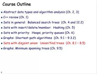
Course Outline • C++ Review (Ch. 1) • Algorithm Analysis (Ch. 2) • Sets with insert/delete/member: Hashing (Ch. 5) • Sets in general: Balanced search trees (Ch. 4, 12.2) • Sets with priority: Heaps, priority queues (Ch. 6) • Graphs: Shortest-path algorithms (Ch. 9.1 – 9.3.2) • Sets with disjoint union: Union/Find (Ch. 8.1–8.5) • Graphs: Minimum spanning trees (Ch. 9.5) • Sorting (Ch. 7)
Data Structures for Sets • Many applications deal with sets. • Compilers have symbol tables (set of vars, classes) • Dictionary is a set of words. • Routers have sets of forwarding rules. • Web servers have set of clients, etc. • A set is a collection of members • No repetition of members • Members themselves can be sets • Examples • Set of first 5 natural numbers: {1,2,3,4,5} • {x | x is a positive integer and x < 100} • {x | x is a CA driver with > 10 years of driving experience and 0 accidents in the last 3 years}
Set Operations • Unary operation: min, max, sort, makenull, …
Observations • Set + Operations define an ADT. • A set + insert, delete, find • A set + ordering • Multiple sets + union, insert, delete • Multiple sets + merge • Etc. • Depending on type of members and choice of operations, different implementations can have different asymptotic complexity.
Set ADT: Union, Intersection, Difference AbstractDataType SetUID instance multiple sets operations union (s1,s2): {x | x in s1 or x in s2} intersection (s1,s21): {x | x in s1 and x in s2} difference (s1,s2): {x | x in s1 and x not in s2}
Examples • Sets: Articles in Yahoo Science (A), Technology (B), and Sports (C) • Find all articles on Wright brothers. • Find all articles dealing with sports medicine • Sets: Students in CS10 (A), CS20 (B), and CS40 (C) • Find all students enrolled in these courses • Find students registered for CS10 only • Find students registered for both CS10 and CS20 • Etc.
Set UID Implementation: Bit Vector • Set members known and finite (e.g., all students in CS dept) • Operations • Union: u[k]= x[k] | y[k]; • Intersection: u[k] = x[k] & y[k]; • Difference: u[k] = x[k] & ~y[k]; • Complexity: O(n): n size of the set students 1 0 1 1 0 0 1 A set 0 1 1 1 1 courses
Set UID Implementation: linked lists • Bit vectors great when • Small sets • Known membership • Linked lists • Unknown size and members • Two kinds: Sorted and Unsorted
Set UID Complexity: Unsorted Linked List • Intersection For k=1 to n do Advance setA one step to find kth element; Follow setB to find that element in B; If found then Append element k to setAB End • Searching for each element can take n steps. • Intersection worst-case time O(n2).
Set UID Complexity: Sorted Lists • The list is sorted; larger elements are to the right • Each list needs to be scanned only once. • At each element: increment and possibly insert into A&B, constant time operation • Hence, sorted list set-set ADT has O(n) complexity • A simple example of how even trivial algorithms can make a big difference in runtime complexity.
Set UID: Sorted List Intersection • Case A *setA=*setB • Include *setA (or *setB ) in *setAB • Increment setA • Increment setB • Case B *setA<*setB • Increment setA Until • *setA=*setB (A) • *setA>*setB (C) • *setA==null • Case C *setA>*setB • Increment setB Until • *setA=*setB (A) • *setA<*setB (B) • *setB==null • Case D *setA==null or *setB==null • terminate
Dictionary ADTs • Maintain a set of items with distinct keys with: • find (k): find item with key k • insert (x): insert item x into the dictionary • remove (k): delete item with key k • Where do we use them: • Symbol tables for compiler • Customer records (access by name) • Games (positions, configurations) • Spell checkers • Peer to Peer systems (access songs by name), etc.
Naïve Implementations • The simplest possible scheme to implement a dictionary is “log file” or “audit trail”. • Maintain the elements in a linked list, with insertions occuring at the head. • The search and delete operations require searching the entire list in the worst-case. • Insertion is O(1), but find and delete are O(n). • A sorted array does not help, even with ordered keys. The search becomes fast, but insert/delete take O(n).
Hash Tables: Intuition • Hashing is function that maps each key to a location in memory. • A key’s location does not depend on other elements, and does not change after insertion. • unlike a sorted list • A good hash function should be easy to compute. • With such a hash function, the dictionary operations can be implemented in O(1) time.
One Simple Idea: Direct Mapping Perm # Student Records Graduates
Hashing : the basic idea • Map key values to hash table addresseskeys -> hash table address This applies to find, insert, and remove • Usually: integers-> {0, 1, 2, …, Hsize-1}Typical example: f(n) = n mod Hsize • Non-numeric keys converted to numbers • For example, strings converted to numbers as • Sum of ASCII values • First three characters
Hashing : the basic idea Student Records Perm # (mod 9) Graduates
Hashing: • Choose a hash function h; it also determines the hash table size. • Given an item x with key k, put x at location h(k). • To find if x is in the set, check location h(k). • What to do if more than one keys hash to the same value. This is called collision. • We will discuss two methods to handle collision: • Separate chaining • Open addressing
Maintain a list of all elements that hash to the same value Search -- using the hash function to determine which list to traverse Insert/deletion–once the “bucket” is found through Hash, insert and delete are list operations Separate chaining 0 1 2 3 4 5 6 7 8 9 10 23 1 56 24 36 14 16 17 7 29 31 20 42 find(k,e) HashVal = Hash(k,Hsize);if (TheList[HashVal].Search(k,e))then return true;else return false; class HashTable { …… private: unsigned int Hsize; List<E,K> *TheList; ……
Insertion: insert 53 0 1 2 3 4 5 6 7 8 9 10 0 1 2 3 4 5 6 7 8 9 10 23 1 56 23 1 56 24 24 36 14 36 14 16 16 17 17 7 29 7 29 53 20 42 31 20 42 31 53 = 4 x 11 + 9 53 mod 11 = 9
Analysis of Hashing with Chaining • Worst case • All keys hash into the same bucket • a single linked list. • insert, delete, find take O(n) time. • Average case • Keys are uniformly distributed into buckets • O(1+N/B): N is the number of elements in a hash table, B is the number of buckets. • If N = O(B), then O(1) time per operation. • N/B is called the load factor of the hash table.
If collision happens, alternative cells are tried until an empty cell is found. Linear probing :Try next available position Open addressing 0 1 2 3 4 5 6 7 8 9 10 42 1 24 14 16 28 7 31 9
Linear Probing (insert 12) 0 1 2 3 4 5 6 7 8 9 10 42 1 24 14 16 28 7 0 1 2 3 4 5 6 7 8 9 10 42 1 31 24 9 14 12 16 28 7 31 9 12 = 1 x 11 + 1 12 mod 11 = 1
Search with linear probing (Search 15) 0 1 2 3 4 5 6 7 8 9 10 42 1 24 14 12 16 28 7 31 9 15 = 1 x 11 + 4 15 mod 11 = 4 NOT FOUND !
Search with linear probing // find the slot where searched item should be in int HashTable<E,K>::hSearch(const K& k) const { int HashVal = k % D; int j = HashVal; do {// don’t search past the first empty slot (insert should put it there) if (empty[j] || ht[j] == k) return j; j = (j + 1) % D; } while (j != HashVal); return j; // no empty slot and no match either, give up } bool HashTable<E,K>::find(const K& k, E& e) const { int b = hSearch(k); if (empty[b] || ht[b] != k) return false; e = ht[b]; return true; }
Deletion in Hashing with Linear Probing • Since empty buckets are used to terminate search, standard deletion does not work. • One simple idea is to not delete, but mark. • Insert: put item in first empty or marked bucket. • Search: Continue past marked buckets. • Delete: just mark the bucket as deleted. • Advantage: Easy and correct. • Disadvantage: table can become full with dead items.
Deletion with linear probing: LAZY (Delete 9) 0 1 2 3 4 5 6 7 8 9 10 0 1 2 3 4 5 6 7 8 9 10 42 42 1 1 24 24 14 14 12 12 16 16 28 28 7 7 31 31 D 9 9 = 0 x 11 + 9 9 mod 11 = 9 FOUND !
Eager Deletion: fill holes • Remove and find replacement: • Fill in the hole for later searches remove(j) { i = j; empty[i] = true; i = (i + 1) % D; // candidate for swapping while ((not empty[i]) and i!=j) { r = Hash(ht[i]); // where should it go without collision? // can we still find it based on the rehashing strategy? if not ((j<r<=i) or (i<j<r) or (r<=i<j)) then break; // yes find it from rehashing, swap i = (i + 1) % D; // no, cannot find it from rehashing } if (i!=j and not empty[i]) then { ht[j] = ht[i]; remove(i); } }
Eager Deletion Analysis (cont.) • If not full • After deletion, there will be at least two holes • Elements that are affected by the new hole are • Initial hashed location is cyclically before the new hole • Location after linear probing is in between the new hole and the next hole in the search order • Elements are movable to fill the hole Initial hashed location Location after linear probing Initial hashed location Next hole in the search order New hole Next hole in the search order
Eager Deletion Analysis (cont.) • The important thing is to make sure that if a replacement (i) is swapped into deleted (j), we can still find that element. How can we not find it? • If the original hashed position (r) is circularly in between deleted and the replacement i r j r i Will not find i past the empty green slot! j r i i r j Will find i j i i r r
Quadratic Probing • Solves the clustering problem in Linear Probing • Check H(x) • If collision occurs check H(x) + 1 • If collision occurs check H(x) + 4 • If collision occurs check H(x) + 9 • If collision occurs check H(x) + 16 • ... • H(x) + i2
Quadratic Probing (insert 12) 0 1 2 3 4 5 6 7 8 9 10 42 1 24 14 16 28 7 0 1 2 3 4 5 6 7 8 9 10 42 1 31 24 9 14 12 16 28 7 31 9 12 = 1 x 11 + 1 12 mod 11 = 1
Double Hashing • When collision occurs use a second hash function • Hash2 (x) = R – (x mod R) • R: greatest prime number smaller than table-size • Inserting 12 H2(x) = 7 – (x mod 7) = 7 – (12 mod 7) = 2 • Check H(x) • If collision occurs check H(x) + 2 • If collision occurs check H(x) + 4 • If collision occurs check H(x) + 6 • If collision occurs check H(x) + 8 • H(x) + i * H2(x)
Double Hashing (insert 12) 0 1 2 3 4 5 6 7 8 9 10 42 1 24 14 16 28 7 0 1 2 3 4 5 6 7 8 9 10 42 1 31 24 9 14 12 16 28 7 31 9 12 = 1 x 11 + 1 12 mod 11 = 1 7 –12 mod 7 = 2
Rehashing • If table gets too full, operations will take too long. • Build another table, twice as big (and prime). • Next prime number after 11 x 2 is 23 • Insert every element again to this table • Rehash after a percentage of the table becomes full (70% for example)
Good and Bad Hashing Functions • Hash using the wrong key • Age of a student • Hash using limited information • First letter of last names (a lot of A’s, few Z’s) • Hash functions choices : • keys evenly distributed in the hash table • Even distribution guaranteed by “randomness” • No expectation of outcomes • Cannot design input patterns to defeat randomness
Examples of Hashing Function • B=100, N=100, keys = A0, A1, …, A99 • Hashing(A12) = (Ascii(A)+Ascii(1)+Ascii(2)) / B • H(A18)=H(A27)=H(A36)=H(A45) … • Theoretically, N(1+N/B)= 200 • In reality, 395 steps are needed because of collision • How to fix it? • Hashing(A12) = (Ascii(A)*22+Ascii(1)*2+Ascci(2))/B • H(A12)!=H(A21) • Examples: numerical keys • Use X2 and take middle numbers
Collision Functions • Hi(x)= (H(x)+i) mod B • Linear pobing • Hi(x)= (H(x)+ci) mod B (c>1) • Linear probing with step-size = c • Hi(x)= (H(x)+i2) mod B • Quadratic probing • Hi(x)= (H(x)+ i * H2(x)) mod B
Analysis of Open Hashing • Effort of one Insert? • Intuitively – that depends on how full the hash is • Effort of an average Insert? • Effort to fill the Bucket to a certain capacity? • Intuitively – accumulated efforts in inserts • Effort to search an item (both successful and unsuccessful)? • Effort to delete an item (both successful and unsuccessful)? • Same effort for successful search and delete? • Same effort for unsuccessful search and delete?
More on hashing • Extensible hashing • Hash table grows and shrinks, similar to B-trees
Issues: • What do we lose? • Operations that require ordering are inefficient • FindMax: O(n) O(log n) Balanced binary tree • FindMin: O(n) O(log n) Balanced binary tree • PrintSorted: O(n log n) O(n) Balanced binary tree • What do we gain? • Insert: O(1) O(log n) Balanced binary tree • Delete: O(1) O(log n) Balanced binary tree • Find: O(1) O(log n) Balanced binary tree • How to handle Collision? • Separate chaining • Open addressing