Lecture 1 3
Lecture 1 3. Shape from Shading. Shape from Shading. Looking at finding normal, not distance Normal: Describe the shape. Assuming point light source is far away p,q are unknowns. Ellipse. SFS: Data Constraint. Given an intensity value I, (p,q) are constrained to be an ellipse. q. p.


Lecture 1 3
E N D
Presentation Transcript
Lecture 13 Shape fromShading
Shape from Shading Looking at finding normal, not distance Normal: Describe the shape Assuming point light source is far away p,q are unknowns Ellipse
SFS: Data Constraint Given an intensity value I, (p,q) are constrained to be an ellipse q p
Self Occluding If know self occluding, we can estimate normal. Normal for self occluding edges are perpendicular to the edge in 2D
SFS In human : tends to assume that light is above
SFS: Classical Work Horn and Schunk Use (p,q) Problem: Self Occluding p,q undefined At occluding edge dz/dx p ∞, q∞ To rectified this, sphere coordinates (,) are used
Photometric Stereo 2/3 lights • Given L1, Observe I1 • Given L2, Observe I2 • Given L3, Observe I3 • Have 3 lights at different directions with distance ∞ • Turn on L1, take pictures • Turn on L2, take pictures • Turn on L3, take pictures
Photometric Stereo I(x,y) = kdId(N.L) = N.L = Albedo = whiteness
Photometric Stereo 4 unknowns : albedo and normal unknown known known
Photometric Stereo I = L.N 1
Remaining Topic • Genetic Algorithm • Neural Network • Motion Processing • Structure • Tracking (Fovea – Center Of Vision) • Camera Calibration • Object Recognition Models
Genetic Algorithm • Optimization Technique Based on “Survival of Fittest” • Population Size – Fixed • Each solution is an individual • Fitness of Individual – Fitness of “Chromosome” (small part) • “Goodness” • Crossover – Combining Parts of 2 or more individuals • New child is put into population. May die. • Mutation – “Random change done to Part of an Individual”
Genetic Algorithm Charls Darwin – “Survival of Fitness” proposed how species develop Moth - Industrial Revolution YellowBlack 99%1% 70%30% 20%80%
Genetic Algorithm Algorithm: • Create a random solution of 20 individuals Sort by fitness { (1,__), (2, __), (3, __), …. } • R = Random(0,1) if (R<0.9) /* Cross Over */ Use 2 or more solutions to create new one else Create a new random Individual Insert new individual in to population if it is fitter than the worst one Repeat Until the top 20 does not change
Problem Statement: Input • The Order Book consists of Many Instances of a Set of Patterns • Each Piece of garment can be placed at 0 degrees or 180 degrees
W L Problem Statement: Output • Place all the pieces in the order book to use minimum fabric • length on a fixed width roll • Method: Genetic Algorithm
About Genetic Algorithms • An optimization method that mimics the evolution of life using concepts of survival of the fittest within a fixed population. • Parts of Genetic Algorithm: • Individual – a solution with known fitness • Population – set of individuals forming the genetic pool • Fitness Function – a measure of the goodness of an individual • Creating a New Individual through Reproduction: 1. Self Replication 2. Crossover 3. Mutation • Output, result reported as the most fit individual in population.
Related Work: Pargas and Jain 1993 [8] R. P. Pargas and R. Jain. A Parallel Stochastic Optimization Algorithm for Solving 2D Bin Packing Problems. IEEE Int. Conf. on A.I. for Applications. 1993. • A stochastic approach to bin packing 2-D figures • Similar to genetic algorithms and simulated annealing • Has 80% efficiency on regular shapes • Tested on objects that can be packed to 100% efficiency • For garments, efficiency cannot be 100% • We compare to human expert for benchmark
G. Roussel and S. Maouche, “Improvements About Automatic Lay-Planning For Irregular Shapes on Plain Fabric” IEEE Proc. Systems Man and Cybernetics, System Engineering, 1993. Shape layout problem for garment pieces Use a heuristic tree search algorithm called -admissible algorithm Reasonable results Too much time spent back-tracking Tends to have a local minimum problem Related Work: Roussel and Mouche 1993 [9]
H.S. Ismail and K.B. Hon. The Nesting of two-dimensional Shapes Using Genetic Algorithms. Proceedings of The Institution of Mechanical Engineers Part B, Journal of Engineering Manufacture. 1995. Minimize Raw Mat for cutting 2-D pieces Uses Genetic Algorithms and Heuristics Simple shapes used Raw Material width not fixed, unrealistic Related Work: Ismail and Hon [11]
Related Work: Bounsaythip et al [10] C. Bounsaythip, S. Maouche and M. Neus. Evolutionary Search Techniques Application in Automated Lay-Planning Optimization Problem. IEEE Int. Conf. on Intelligent Systems for the 21st Century, 1995. • Minimize unoccupied space by Evolutionary Algorithm • Shape representation by Comb Code • Efficiency Measure: Length of Raw Mat (Fabric). • Used pant garment pieces, regular shapes • Good Results due to regular shapes used.
Related Work: Bounsaythip and Maouche [12] C. Bounsaythip and S. Maouche. Irregular Shape Nesting And Placing With Evolutionary Approach”. IEEE Int. Conf. On Systems Man and Cybernetics.1997. • Use the comb code representation for each garment piece • Shape placement represented as hierarchical tree • Allow orientations of 0, 90, 180, and 270 degrees • Crossover: combine parts of tree, removing redundancy • Results presented on relatively simple shapes, making it difficult to assess the efficiency achieved
Placing Items from Order Book 1 2 3 4 5 6 7 8 9 10 11 12 13 14 • The Order Book consists of Many Instances of a Set of Patterns • Each Piece of garment can be placed at 0 degrees or 180 degrees • Each garment piece is polygonal • Smooth contours (splines) approximated by convex hull first
Placement Method: Check for Overlaps Convex Polygons Assumed Upon placing a new polygon, must check that: 1. NO vertex is INSIDE other polygons 2. NO other polygon’s vertex is INSIDE
Our Genetic Algorithm • 1. Set and Randomly Initialize the Population of size P = 15 • Divide Individual into chromosome strips. Compute strip efficiency. • 3. Crossover, Mutation, and Selection: • Repeat • If random (0, 1) < crossover probability • Create a New Individual by Crossover: • Repeat • Sample for a chromosome from the solution biased by efficiency • Recompute chromosome efficiency based on Order Book balance • Until No Efficient Chromosome Available • Fill Remaining Solution Randomly by Order Book balance • Else • Create New Individual by Mutation: Fill Randomly from Order Book • Insert the solution into the new population • Check for Survival of Fittest P = 15 • Until(Population has converged)or(No improvement in Best Solution)
5 3 4 2 1 7 Step 1: Initial Random Population An Individual Solution: S = [(F1, O1), (F2, O2),…,(Fn, On), L)] whereS - completed order book Fi - garment piece number Oi - orientation at 0 or 180 degrees L - Length of Fabric used S1 = [(5, 1), (3, 0), (4, 1), (1, 1), (2, 0), 15] S2 = [(1, 0), (3, 0), (2, 1), (3, 0), (4, 0), 17] S3 = [(5, 1), (3, 0), (7, 1), (1, 1), (2, 0), 20] S4 = [(1, 0), (5, 0), (4, 0), (3, 1), (2, 0), 21] S5 = [(1, 0), (3, 0), (5, 0), (2, 1), (4, 0), 23] S6 = [(4, 0), (5, 0), (1, 1), (2, 0), (3, 0), 25] S7 = [(3, 1), (4, 0), (5, 1), (2, 0), (1, 0), 27] S8 = [(5, 1), (4, 0), (3, 1), (2, 1), (1, 0), 29] S9 = [(3, 0), (2, 0), (1, 0), (5, 1), (4, 1), 32] S10 = [(4, 1), (3, 0), (1, 1), (2, 1), (5, 1), 34]
Lstr1 Lstr2 Lstr3 W L Step 2: Determine Strips Each Strip is determined by largest piece along column. Efficiency of each strip is Computed, used for crossover
LB P = LB Crossover: Sampling Within Population
EB P = EB Crossover: Sampling for Efficient Strips • After sampling from population for 4 best solutions, Crossover takes place using efficient strips first
high lowered Crossover: Efficiency Decreases over Time • Efficiency decreases as Order Book fills up • Once Efficiency too low, fill remaining items randomly
Mutation: New Random Individual • When Efficiency low, fill randomly is partly like mutation • Mutation by generating a new random solution • This new individual usually does not survive • Our results are compared with layout by human expert
Experimental Result 1: Rectangles 6 Sets in Order Book G.A.: 1:15 Hrs.
Rectangles by Human Expert Manually: 0:25 Hrs.
Experimental Result 2: Shirt Pieces 10 Sets in Order Book
Shirt Pcs. (10 orders) by G.A. G.A.: 51:08 Hrs.
Shirt Pcs. (10 orders) by Human Manually: 1:25 Hrs.
Experimental Result 3: Multi-Edged Shapes by G.A. 3 Sets in Order Book
Multi-Edged G.A. vs. Human G.A.: 0:57 Hrs.
Finding Crossover Number 62 E % 3 1 60 2 4 58 5 56 54 52 0 5 10 15 20 25 30 35 40 45 50 55 60 65 70 75 Iterations
Finding Good Population Size 62 E % 30 25 60 15 58 10 20 56 54 52 50 0 5 10 15 20 25 30 35 40 45 50 55 60 65 70 75 Iterations
high lowered Discussion and Conclusion • Main Problem: successive crossover reduces efficiency of good strips. • Efficiency 3-5% lower than human expert, while taking more time. • Efficiency depends on the complexity of the piece, making it hard to compare results among researchers.