Download
1 / 31
330 likes | 450 Views
This article delves into the principles of database normalization, discussing why normal forms are important in database design. It covers the roles of First Normal Form (1NF), Second Normal Form (2NF), and Third Normal Form (3NF) in reducing redundancies and improving data integrity. The text outlines key concepts such as atomic attributes, functional dependencies, and the trade-offs between redundancy and efficiency. Examples illustrate how to transform unnormalized relations into well-structured databases, contributing to better data management and maintenance.

E N D
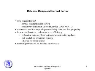
Database Design and Normal Forms • why normal forms? • - format standardization (1NF) • - reduction/elimination of redundancies (2NF, 3NF, ...) • theoretical tool for improving/maintaining database design quality • in practice, however: redundancy vs. efficiency • - redundant data may lead to inconsistencies after updates • - but useful for efficiency reasons • (shorter response times) • tradeoff problem: to be decided case by case O. Günther: Database Management Systems
1st Normal Form (1NF) • all attributes have to be atomic • no „repeating groups“ • important foundation of the relation model • but: may lead to increased redundancy • Ex.: relation Supplies (a) not in 1NF (b) in 1NF repeating groups O. Günther: Database Management Systems
1NF + for all attributes A and attribute sets X in relation R: • X A in R X is no real subset of at least one key of R • AND OR • A not in X A is key attribute (i.e., it belongs to at least one key of R) • note: if R has only one key, this is equivalent to: • 1 NF + each non-key attribute is fully functionally dependent on the key, • i.e., it can not be inferred from part of the key • trivially true for one-column keys • Ex.: relation Supplies • - Supplies (Name, Product, Price) is in 2NF if and only if Price • depends on both Name and Product (free pricing) • - with fixed prices (e.g. books in Germany), Supplies is no longer in 2NF • - possibly decomposition into Supplies’ (Name, Product) and • Costs (Product, Price) 2nd Normal Form (2NF) O. Günther: Database Management Systems
2NF + for all attributes A and attribute sets X in relation R: • X is a key of R • X A in R OR • AND X contains a key of R • A not in X OR • A is a key attribute • note: if there is only one key, this is equivalent to: • 2NF + non-key attributes are mutually independent • sufficient (but not necessary) condition:: • if an FD in the minimal cover contains all attributes of R then R is in 3NF • Ex.: relation Customers (Name, Address, Balance) • - all attributes atomic 1NF • - keys have only one column 2NF • - Address and Balance are mutually independent 3NF 3rd Normal Form (3NF) O. Günther: Database Management Systems
3NF - An Example • relation R = (C, S, Z) • functional dependencies: F = { CS Z, Z C} • R in 3NF? • keys of R: • key attributes of R: • 1NF • 2NF • 3 NF O. Günther: Database Management Systems
3NF - An Example • relation R = (C, S, Z) • functional dependencies: F = { CS Z, Z C} • R in 3NF? • keys of R: CS, ZS • key attributes of R: • 1NF • 2NF • 3 NF O. Günther: Database Management Systems
3NF - An Example • relation R = (C, S, Z) • functional dependencies: F = { CS Z, Z C} • R in 3NF? • keys of R: CS, ZS • key attributes of R: C, S, Z • 1NF • 2NF • 3 NF O. Günther: Database Management Systems
3NF - An Example • relation R = (C, S, Z) • functional dependencies: F = { CS Z, Z C} • R in 3NF? • keys of R: CS, ZS • key attributes of R: C, S, Z • 1NF: no problem • 2NF • 3 NF O. Günther: Database Management Systems
3NF - An Example • relation R = (C, S, Z) • functional dependencies: F = { CS Z, Z C} • R in 3NF? • keys of R: CS, ZS • key attributes of R: C, S, Z • 1NF: no problem • 2NF: o.k. because Z and C are key attributes • 3 NF O. Günther: Database Management Systems
3NF - An Example • relation R = (C, S, Z) • functional dependencies: F = { CS Z, Z C} • R in 3NF? • keys of R: CS, ZS • key attributes of R: C, S, Z • 1NF: no problem • 2NF: o.k. because Z and C are key attributes • 3 NF: o.k. for the same reason O. Günther: Database Management Systems
Decompositon into 3NF • given: relation R, set of FD's F • find: decomposition of R into a set of 3NF relations Ri • algorithm: • IF R in 3NF • THEN stop • ELSE • compute minimal cover F of F; • create a separate relation Ri = A for each attribute Athat does not • occur in any FD in F; • create a relation Ri = XA for each FD X A in F; • if the key K of R does not occur in any relation Ri, create one • more relation Ri = K. • decomposition fulfills • - lossless join • - preservation of dependencies O. Günther: Database Management Systems
Decomposition into 3NF - Example Attributes: L ... Lecture R ... Room I ... Instructor S ... Student T ... Time G ... Grade Relational Schema: R= (L, I, T, R, S, G) Functional Dependencies: O. Günther: Database Management Systems
Decomposition into 3NF - Example (cont.) Attributes: L ... Lecture R ... Room I ... Instructor S ... Student T ... Time G ... Grade Relational Schema: R= (L, I, T, R, S, G) Functional Dependencies: F = { L I , TR L, TI R, LS G, TS R, TRI LR} O. Günther: Database Management Systems
Decomposition into 3NF - Example (cont.) • Keys: • Key Attributes: O. Günther: Database Management Systems
Decomposition into 3NF - Example (cont.) • Keys: ST • Key Attributes: S, T O. Günther: Database Management Systems
Decomposition into 3NF - Example (cont.) • F = { L I , • TR L, • TI R, • LS G, • TS R, • TRI LR} • Minimal Cover • Decomposition into Ri O. Günther: Database Management Systems
Decomposition into 3NF - Example (cont.) • F = { L I , • TR L, • TI R, • LS G, • TS R, • TRI LR} • Minimal Cover • F = {L I , • TR L, • TI R, • LS G, • TS R} • Decomposition into Ri O. Günther: Database Management Systems
Indices • data structures (often tree structures) that serve to accelerate database searches • frequent synonyms: index structures, access methods • Ex.: Supplies (Name, Product, Price) O. Günther: Database Management Systems
Indices (cont.) • Name and Product are the indexed columns • Index on Name is primary index • - indexed column is part of the primary key • - relation is sorted by increasing primary key • - well suited for processing range queries (Ex.: Find all suppliers • whose name starts with B, C or D) • all other indices: secondary indices • tradeoff: queries vs. updates • - indices accelerate many queries ... • - ... but slow down updates O. Günther: Database Management Systems
Dense vs. Sparse Indices • relations are stored in blocks (pages) on the magnetic disk • crucial cost factor: how many blocks to I have to transfer from disk • to main memory in order to answer the query? • non-dense (or sparse) index: one index entry per block • - for a primary index it suffices to store the smallest key value per block • - index supports the system when looking for the relevant block(s) • - inside each block: local search (cf. telephone directory) • - useful for large relations because very compact • - only possible for columns according to which the relation • has been sorted (cf. phone directory) • - therefore: at most one sparse index per relation • dense index: one index entry per tuple O. Günther: Database Management Systems
How Does a Disk Access Work? Disk Drive Read block Main Memory Write block O. Günther: Database Management Systems
Indexon Name (sparse) Index on Product (dense) Dense vs. sparse indices: An Example Price Oysters Peanuts Oysters Peanuts Lettuce Lettuce O. Günther: Database Management Systems
Layered Indices • large relations large indices • indexing a larger index leads to a smaller index etc. • tree structure • root fits on one page (= one block) Index (often dense) File (Relation) O. Günther: Database Management Systems
B+ Tree • tree structure as described above A O. Günther: Database Management Systems
B+ Tree(cont.) • B+ trees are balanced (i.e., all leaves are on the same level) • lowest level (leaves): dense, otherwise : sparse • each node fits on one page ( N entries) • N = page size / space requirements per entry (Ex. above: N = 3) • minimal page utilization (guaranteed): N/2 entries O. Günther: Database Management Systems
B+ Tree (cont.) • each node has between N/2 and N entries • problems: overflow, underflow • Ex.: N = 3 A O. Günther: Database Management Systems
B+ Tree (cont.) O. Günther: Database Management Systems
B+Baum (cont.) O. Günther: Database Management Systems
Hashing - An Alternative to Indices • hash function h: • data value storage address • Ex.: storage address = data value MOD p • (p typically a prime number) • Ex.: p = 13 Hash Field O. Günther: Database Management Systems
Hashing (cont.): Storage Structure • only one hash field per relation! • advantage: very fast access • disadvantage: • - relation dispersed across the disk • - collisions O. Günther: Database Management Systems
Hashing (cont.): Collision Chains O. Günther: Database Management Systems