Multimedia Data Access
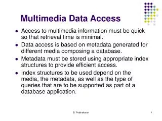
Multimedia Data Access. Access to multimedia information must be quick so that retrieval time is minimal. Data access is based on metadata generated for different media composing a database. Metadata must be stored using appropriate index structures to provide efficient access.

Multimedia Data Access
E N D
Presentation Transcript
Multimedia Data Access • Access to multimedia information must be quick so that retrieval time is minimal. • Data access is based on metadata generated for different media composing a database. • Metadata must be stored using appropriate index structures to provide efficient access. • Index structures to be used depend on the media, the metadata, as well as the type of queries that are to be supported as part of a database application. B. Prabhakaran
Text Metadata • Text metadata: index features that occur in a document as well as descriptions about the document. • Choice of index features: should describe the documents in a possibly unique manner. • Definitions document frequency and inverse document frequency describe the characteristics of index features. • Document frequency df(øi) of an indexing feature øi : the number of documents in which the indexing feature appears • df(øi) = |{dj εD | ff(øi, dj) > 0| B. Prabhakaran
Document Frequency • Document frequency df(øi) of an indexing df(øi) = |djεD | ff(øi, dj) > 0| • dj refers to the jth document where the document index occurs • D is the set of all documents • ff(øi, dj) is the feature frequency. • Feature frequency denotes the number of occurrences of the indexing feature øi in a document dj . B. Prabhakaran
Inverse Document Frequency • Inverse Document Frequency idf(øi) of an indexing feature øi describes its specificity. • idf(øi) = log((n+1) / df(øi) + 1), where n denotes the number of documents in a collection. • Selection of an indexing feature: • df(øi) is below an upper bound, so that the feature appears in less number of documents thereby making the retrieval process easier. • Implies that the inverse document frequency idf(øi) for the selected index feature øi will be high. B. Prabhakaran
Full Text Scanning • Query feature is searched in the entire set of documents. • For boolean queries (where occurrences of multiple features are to be tested), it might involve multiple searches for different features. • Finite State Machine based approach: Defining a Failure function that is consulted when the Goto function reports fail. • The failure function defines the transition from a state to another state, on receipt of the fail message. • After this failure transition, the Goto function for the new state with the same input symbol is executed. B. Prabhakaran
Full Text Scanning B. Prabhakaran
Inverted Files • Store search information about a document or a set of documents. • Search information includes the index feature and a set of postings. • Postings point to the set of documents where the index features occur. • An inverted file is based on a single key and hence efficient access to the index features should be supported. • Index features can be sorted alphabetically or stored in the form of a hash table or using sophisticated mechanism such as B-trees. B. Prabhakaran
Inverted Files .. B. Prabhakaran
Hash Tables for Inverted Files • Inverted indices can also be stored in the form of a hash table. • A hashing function is used to map the index features that are in the form of characters or strings, into hash table locations. B. Prabhakaran
Multimedia Indexing B. Prabhakaran
Signature Files • Query for searching a text document consists of more than one feature: • different techniques must be used to search the information. • Query: `Multimedia database management systems' • Each attribute hashed to give a bit pattern of fixed length • Bit patterns for all the attributes are superimposed (Boolean OR operation) to derive the signature value of the query. B. Prabhakaran
Signature Files • Query for searching a text document consists of more than one feature: • different techniques must be used to search the information. • Query: `Multimedia database management systems' • Each attribute hashed to give a bit pattern of fixed length • Bit patterns for all the attributes are superimposed (Boolean OR operation) to derive the signature value of the query. B. Prabhakaran
Signature Files • Query: `Multimedia database management systems' • Multimedia 100 010 001 011 • Database 010 001 100 010 • Management 001 100 010 001 • System 110 011 101 011 • Signature 111 111 111 011 • Signature value 111 111 111 011} used as the search information for retrieving the required text document with index features multimedia database management system. B. Prabhakaran
Multimedia Indexing B. Prabhakaran
Clustering Text Files • Clustering or grouping of similar documents accelerates the search • since closely associated documents tend to be relevant to the same requests. • Index features and the search query are viewed as points of a m-dimensional space. Document descriptor dj is defined as, dj = (a1,j, ... , am,j), • m represents the number of indexing features • ai,j represents the weight associated with each feature. • Weights must be high if the feature characterizes the document well and low if the feature is not very relevant for the document. B. Prabhakaran
Clustering Text Files .. • Clusters, c1,..., cn, can be the set of index features used to characterize the document set. • E.g., c1 can represent the documents where the index feature multimedia occurs. • Weights associated with the documents d1 and d3 denote the relevance of the feature multimedia for the two documents. • If d3's association with the feature multimedia is marginal, then the weight associated with (d3, c1) will be very low. B. Prabhakaran
Text Files Clusters B. Prabhakaran
Weight Functions • Binary document descriptor : Presence of a feature by 1 and absence by 0. • Feature frequency, ff(øj,dj). • Document frequency, df(øj). • Inverse document frequency or the feature specificity, idf(øj). • ff(øj,dj}) * Rj, where Rj is the feature relevance factor for a document j. • Values for the above weight functions have to be estimated for generating document clusters. • Weight functions based on binary document descriptor, feature frequency, document frequency and inverse document frequency are straight forward. B. Prabhakaran
Multimedia Indexing B. Prabhakaran
Learning-based Weight Functions • Many of the learning-based methods are probabilistic in nature. • Learning approaches have two phases : • Learning phase • Application phase • Learning phase: a set of learning queries are used to derive a feedback information. • Learning queries are similar to the ones used normally for text access. Applied to a specific document or a set of documents. • Based on the relevance of these queries for selecting documents: • Probabilistic weights are assigned to the indexing features or to the documents (or both). B. Prabhakaran
Learning-based Weight Functions • Application phase: Normal queries are answered based on the weights estimated during the learning phase. • Feedback information can also be derived from the normal queries for modifying the associated weights (as indicated by the double headed arrows for normal queries in accompanying Figure). • Following methods are normally used for deriving the feedback information. • Binary Independence Indexing • Darmstadt Indexing Approach • Text Retrieval From Document Clusters B. Prabhakaran
Binary Independence Indexing • Probabilities for indexing features are estimated during a learning phase. • In this learning phase, sample queries for a specific document dj are analyzed. • Based on the indexing features present in the sample queries, the probabilistic weights for each feature is determined. • Disadvantage: feedback information derived from the sample set of queries is used for processing all the queries that occur. • Since sample set of queries cannot reflect the nature of all possible queries, weights derived using this type of feedback may not be accurate. B. Prabhakaran
Darmstadt Indexing Approach • Difference: feedback information is derived during the learning phase as well as the application phase. • Hence, new documents and new index features can be introduced into the system. • System derives the feedback information continuously and applies it to the newly introduced components (documents or index features). • Since size of the learning sample continually increases over the period of operation, estimates of the weight functions can be improved. B. Prabhakaran
Text Retrieval From Document Clusters • Text retrieval from document clusters employ a retrieval function • computes the similarity measure of the index features with those described for the stored documents. • Retrieval function depends on the weight functions used to create the document clusters. • Documents are ranked based on the similarity of the query and the documents, and then they are presented to the user. B. Prabhakaran
Speech Metadata • Additional constraints on the choice of the index features: • Number of index features have to be quite small, since the pattern matching algorithms (such as HMM, neural networks model and dynamic time warping) used to recognize the index features are expensive. • Large space is needed for storing different possible reference templates (required by the pattern matching algorithms), for each index feature. • Computation time for training the pattern matching algorithms for the stored templates is high. • For a feature to be used as an index, its document frequency $df(øi)$ should be below an upper bound (as discussed for text metadata). • For speech data, the df(øi) should be above a lower bound, so as to have sufficient training samples for the index feature. B. Prabhakaran
Speech Metadata.. • From the point of view of the pattern matching algorithms and the associated cost: • Words and phrases are too large a unit to be used as index features for speech. • Hence, sub-word units can be used as speech index features. • Identifying and using the index features. • Determine the possible sub-word units that can be used as speech index feature • Based on the document frequency values df(øi), select a reasonable number (say, around 1000) index features • Extract different pronunciations of each index feature from the speech document • Using the different pronunciations, train the pattern matching algorithm for identifying the index features B. Prabhakaran
Speech Data Retrieval • Retrieval of speech documents: done by matching the index features given for searching and the ones available in the database. • E.g., if we are to use HMMs as the pattern matching algorithm, then each index feature selected using the above criteria are modeled by a HMM. • The HMMs of all the selected index features are grouped to form a background model. • This model represents all the sub-word units that occur as part of the speech data. • Retrieval is done by checking whether a given word or sentence appears in the available set of documents. • The given word or sentence for searching is broken into sub-word units. B. Prabhakaran
Speech Retrieval B. Prabhakaran
Image Metadata • Image metadata: different features such as identified objects, their locations, color, and texture. • Generated metadata has to be stored in appropriate index structures for providing ease of access. • Logical structures for storing the locations and the spatial relationships among the objects in an image. • Similarity cluster generation techniques where images with similar features (such as color and texture) are grouped together such that images in a group are more similar, compared to images in a different group. B. Prabhakaran
Image Logical Structures • Different logical structures are used to store the identified objects in an image and their spatial relationships. • Storing the identified objects involves identification of their geometrical boundaries as well as the spatial relationships among the objects. • Identifying Geometric Boundaries • MBR (Minimum Bounding Rectangle) Representation • Sweep Line Representation • Identifying the Spatial Relationships • 2D-Strings • 2D-C Strings B. Prabhakaran
MBR Representation • Describes an object's spatial location using the minimum sized rectangle that completely bounds an object. • MBR concept is very useful in dealing with objects that are arbitrarily complex in terms of their boundary shapes. • Also be useful in identifying the overlaps of different objects, by comparing the coordinates of the respective MBRs. B. Prabhakaran
Sweep Line Representation • A Plane Sweep technique is used where a horizontal line and a vertical line sweep the image from top to bottom (horizontal sweep) and from left to right (vertical sweep). • A set of pre-determined points in the image called event points are selected so as to capture the spatial extent of the objects in the image. • Horizontal and vertical sweep lines stop at these event points, and the objects intersected by the sweep line are recorded. • Facial features such as eyes, nose, and mouth are represented by their polygonal approximations. • Vertices of these polygons constitute the set of event points. • Horizontal sweep line (top to bottom): eyes, nose and mouth. • Vertical sweep line (left to right): left eye, mouth, nose and right eye. B. Prabhakaran
2D-Strings • 2D-strings is used to represent the spatial relationships among objects in an image by representing the projection of the objects along the x and y axes. • Objects are assumed to be enclosed by a MBR with their boundaries parallel to the horizontal (x-) and the vertical (y-) axis. • Reference points of the segmented objects are the projection of the objects' centroids on the x- and the y- axis. • Let S := {O1, O2, ..., On} be a set of symbols of the objects that appear in an image. • Let R := {=, <, :} be a set of relation operators. B. Prabhakaran
2D-Strings.. • Let R := {=, <, :} be a set of relation operators. • = At the same spatial location • < To the west of or to the south of (depending on x- & y- axis). • : In the same set as • A 2D-string is represented as two substrings separated by a comma (,). • First substring describes the spatial relationships along the x axis and the second substring the relationships along the y axis. • Consider the facial image: S = {LE, RE, N, M}, where LE is the left eye, RE the right eye, N the nose, and M the mouth. • 2D string for this spatial image is : {LE < N : M < RE, • M < N < LE : RE}. B. Prabhakaran
2D-Strings.. • 2D-string representation of almost all facial images will be the same ! This example is used only to illustrate the use of 2D-strings. • A 2D-string can be thought of as the symbolic projection of the identified objects in an image along the x- and y- axis. • Disadvantage of 2D strings: spatial relationships among the objects are represented based on the projection of the objects' centroids onto the x- and y- axis. • Projection of objects' centroids alone do not reflect the complete picture of the spatial organization. B. Prabhakaran
2D-C Strings • Overcomes the disadvantage of 2D-strings by representing spatial relationships among the boundary of objects (instead of objects' centroids as in 2D-strings). • There are thirteen possible relationships between two rectangles that enclose the objects (ignoring the rectangles' length information) along the $x-$(or $y-$)-axis. B. Prabhakaran
Retrieval Based Spatial Relationships • In the case of sweep line representation of the spatial relationships, the sweep line representation is generated for the query image also. • If the generated representation for the query image matches the one(s) stored in the database, then the image(s) is(are) retrieved. • For techniques such as 2D- or 2D-C string, pre-processing is required to translate the string description of each image into a set of the form: • {Oi, Oj, rij}. Oi, Oj represent the objects and rij represents the rank of the Oi with respect to Oj. • Rank rij for the 2D-string is defined as an integer value between 1 and 9, i.e., 1≤ rij≤ 9. B. Prabhakaran
Retrieval Based Spatial Relationships .. • Rank of the object depends on the position of one object with respect to another. • Rank of Oi with respect to Oj is 8. Basically, rank 1 represents north of, rank 2 represent north-west of and so on. • Another e.g., facial image: rank of LE (left eye) with respect to RE (right eye) is 3. B. Prabhakaran
Retrieval Based Spatial Relationships … • Based on the ranks among the different possible combinations of the objects, the set of the {Oi, Oj, rij} can be derived. • Derived set stored in the database for each image. • For the query image, a similar set is derived. • A set intersection operation is carried out between the set for the query image and the sets stored in the database. • A non-empty intersection implies similarity among the images. • Subset having more number of elements in the intersection set being more similar to the queried image. B. Prabhakaran
Image Clustering • Features such as color and texture of an image can be indexed using similarity cluster generation methodologies. • Mapping function is defined to generate a similarity measure based on the features to be indexed. • Images are then grouped in such a way that: • Difference between the similarity measures of the images within a cluster are below a known upper bound. • Mapping function F maps an image to a point in the 2-dimension similarity space: • Hence, a query trying to retrieve image by similarity within a distance d becomes a circle of radius d in the 2-dimensional similarity space. B. Prabhakaran
Multimedia Indexing B. Prabhakaran
Image Clustering … • Dimension of the similarity space can be the same as the number of features used, calling it a f-d space. • Point onto which an image is mapped in the f-d space is called a f-d point. • Define a mapping function F for the features based on which images are to be indexed • Use of spatial access structure to group the f-d points and to store them as clusters • Mapping function should be able to map an image to a f-d point in the similarity space. • It should also be able to preserve the distance between two images. B. Prabhakaran
Image Clustering … • Preserving distance between two images: • Assume dissimilarity between two images can be expressed as quantity D. • Mapping function should map the two images onto the similarity space such that the two points are a distance δapart, δαD. • Preserving the distance in the similarity space makes sure that two dissimilar images cannot be misinterpreted as similar. • Mapping functions depend on the feature to be indexed: color, texture, etc. B. Prabhakaran
Color Mapping Function • Similarity between two images can be estimated based on extracted color features as well as the spatial locations of the color components in the images. • Spatial information implies the positions of pixels having the same color. • Most of the color mapping functions work on the extracted color features and do not consider the spatial information. • Extracted color features are stored in the form of histograms. B. Prabhakaran
Color Mapping Function • Based on intersection of color histograms, to determine whether two images are similar in colors. • Sim(I1,I2) = ∑i=1b min(I1i,I2i) / ∑i=1b I2i • Sim(I1, I2) is the distance between the two images I1 and I2 in the similarity space, I1i and I2i are the number (or the percentage) of pixels in the ith color bin of images of I1 and I2 respectively. B. Prabhakaran
Color Mapping Function • b denotes the number of color bins describing the color shades that are distinguished by the histogram. • Two exactly similar images have a similarity measure of 1. • E.g., images shown in earlier figure: have pixels in adjacent color bins but not in the same bins. • min(I1i,I2i) is zero for all the color bins i. • Disadvantage with this similarity measure: • only the number of pixels in the same color bin are compared. Does not consider the correlation among the color bins. • In the above example, if we assume that adjacent color bins represent shades of a similar color, then the two images might be more similar looking. B. Prabhakaran
Using Correlation Function • Not fair to give the two images a similarity measure of zero. • To take into consideration similarity among different color shades, a similarity measure taking into account the correlation among the colors can be used. • Sim (I1, I2) = ∑i=1b∑ j=1b aij(I1i - I2j)(I1j - I2i) • aij: correlation function defining the similarity between the ith and jth colors. • Other terms are the same as defined in the previous mapping function. • E.g, for the earlier color histograms shown, let us assume that aij is 0.5 for adjacent color bins and 0 for other bins. • Then, similarity measure will be 0.190. B. Prabhakaran
Texture Mapping Functions • Texture features such as coarseness, contrast and directionality are also used to characterize images. • Coarseness is described by terms such as fine, coarse, etc. • Coarseness measure is defined by considering the variations in the gray-levels and elements size. • Contrast is the description of gray level distribution in an image. • Directionality describes the orientation of the patterns that appear in an image. • Cluster generation functions for image textures can be defined in the three dimensional texture space corresponding to coarseness, contrast, and directionality. B. Prabhakaran
Color & Texture Indexing • Techniques described above basically help in mapping the features of images onto points in a similarity space. • These points have to be stored using appropriate access structures so that their fast retrieval can help in fast query processing. • Typically, range trees, called R-trees are used to store this multidimensional space point information. • R-tree is a height-balanced tree, an extension of B-trees for multidimensional objects. • Several variations of R-trees have been proposed in literature. B. Prabhakaran
R-trees • A node in the R-tree can be assumed to represent a minimum bounding rectangle (MBR). • MBR represented by a parent node contains the MBRs represented by it children. • Leaf nodes in the R-trees have pointers to the objects that fall within the MBR represented by the individual nodes. • R-trees can be represented by the tuple (Nt, T, E, bf), corresponding to the following : • Nt represents the non-leaf nodes. These nodes contain entries of the form (l, ptr), where l is the MBR that covers all rectangles in a child node and ptr is a pointer to a child node in the R-tree. B. Prabhakaran

